
AUTOMATIC GENERATION OF OPTIMAL CONTROLLERS
THROUGH MODEL CHECKING TECHNIQUES
Giuseppe Della Penna, Daniele Magazzeni, Alberto Tofani
Dipartimento di Informatica, Universit
`
a di L’Aquila, Italy
Benedetto Intrigila
Dipartimento di Matematica Pura ed Applicata, Universit
`
a di Roma “Tor Vergata”, Italy
Igor Melatti, Enrico Tronci
Dipartimento di Informatica, Universit
`
a di Roma “La Sapienza”, Italy
Keywords:
Controller Synthesis, Controller Optimization, Model Checking, Nonlinear Systems.
Abstract:
We present a methodology for the synthesis of controllers, which exploits (explicit) model checking techniques.
That is, we can cope with the systematic exploration of a very large state space. This methodology can be
applied to systems where other approaches fail. In particular, we can consider systems with an highly non-
linear dynamics and lacking a uniform mathematical description (model). We can also consider situations
where the required control action cannot be specified as a local action, and rather a kind of planning is required.
Our methodology individuates first a raw optimal controller, then extends it to obtain a more robust one. A
case study is presented which considers the well known truck-trailer obstacle avoidance parking problem, in
a parking lot with obstacles on it. The complex non-linear dynamics of the truck-trailer system, within the
presence of obstacles, makes the parking problem extremely hard. We show how, by our methodology, we can
obtain optimal controllers with different degrees of robustness.
1 INTRODUCTION
Control systems (or, shortly, controllers) are small
hardware/software components that control the be-
havior of larger systems, the plants. A controller con-
tinuously analyzes the plant state (looking at its state
variables) and possibly adjusts some of its parame-
ters (called control variables) to keep the system in
a condition called setpoint, which usually represents
the normal or correct behavior of the system.
In the last years, the use of sophisticated controllers
has become very common in robotics, critical systems
and, in general, in the hardware/software embedded
systems contained in a growing number of everyday
products and appliances.
However, since the primary aim of a controller is
to ensure the correct behavior of the controlled plant,
we have to guarantee the efficiency and the robust-
ness of controllers. By efficiency, we mean the capa-
bility of the controller to bring the system to the set
point in the shortest possible time (also called time
optimality). By robustness, we mean the capability of
the controller to perform well when the state variables
vary outside the design range.
Therefore, the verification of these properties is a
crucial task that is being addressed using different for-
mal methodologies (e.g., model checking and theo-
rem proving) developed in different research commu-
nities (e.g., automata theory and artificial intelligence
(Kautz et al., 2006)). In particular, much work is be-
ing done to provide a methodology for the automatic
(or semi–automatic) synthesis of correct controllers
directly from the plant specifications.
However, efficiency and robustness can hardly be
simultaneously fulfilled, especially in critical sys-
tems, where the system dynamics is difficult to un-
derstand and to control.
Therefore a possible approach for approximate a
correct solution, can be to start by synthesizing a very
efficient or even optimal controller and - as a second
step - to make it robust. (Observe, however, that in
case safety is involved, a better approach could be to
choose the best controller in the class of the safe ones
(Lygeros et al., 1999)).
To this aim, in this paper we describe an automatic
methodology composed by:
1. a procedure for the synthesis of an optimal con-
troller;
2. a procedure for the transformation of the optimal
26
Della Penna G., Magazzeni D., Tofani A., Intrigila B., Melatti I. and Tronci E. (2006).
AUTOMATIC GENERATION OF OPTIMAL CONTROLLERS THROUGH MODEL CHECKING TECHNIQUES.
In Proceedings of the Third International Conference on Informatics in Control, Automation and Robotics, pages 26-33
DOI: 10.5220/0001217900260033
Copyright
c
SciTePress

controller into a robust one;
Our methodology exploits explicit model checking
in an innovative way w.r.t the approaches adopted so
far, especially in the AI planning area. In particular,
the first procedure - looking for an optimal solution -
actually can also be considered as a planner. Indeed,
this procedure does not simply individuate a good lo-
cal move, but searches for the best possible sequence
of actions to bring the plant to the setpoint. There-
fore, it can be also used as a planner, though we will
not pursue this point in the paper.
2 CONTROLLER SYNTHESIS
TECHNIQUES
In this section we recall some basic notions about
controller synthesis and describe the main results pre-
sented in this field by the recent research.
2.1 Controller Synthesis
There are a number of well-established techniques for
the synthesis of controller. For short, we mention only
three of them:
1. PID controllers;
2. fuzzy controllers;
3. dynamic programming techniques.
As it well-known (
˚
Astrom K.J, 2005), PID-based
techniques are very effective for linear systems, while
they badly perform w.r.t. non-linear ones. On the con-
trary our technique is able to cope with such systems,
as shown in the case study.
Fuzzy control is well known as a powerful tech-
nique for designing and realizing control systems, es-
pecially suitable when a mathematical model is lack-
ing or is too complex to allow an analytical treatment
(Li and Gupta, 1995; Jin, 2003). However fuzzy rules
correspond to local actions, so that, in general, they
do not result in an optimal controller. Moreover there
are situations where local actions are not viable at all,
and rather a kind of planning is required. For an ex-
ample of such a situation see the case study.
Dynamic programming techniques are very suit-
able for the generation of optimal controllers (Bert-
sekas, 2005; Sniedovich, 1992). Although our
methodology has a dynamic programming flavor, it
can cope with (and it is especially suitable for) very
rough plant descriptions, whose mathematical defini-
tion cannot be adapted to the dynamic programming
preconditions, when the cost function cannot be de-
composed or the system dynamics function cannot be
inverted. Again, see the case study, where a backward
decomposition of the cost function (in this case, the
length of the path) is hard to perform, due to the com-
plexity of the system dynamics function and to the
presence of obstacles. Indeed, we performed a direct
systematic analysis of the trajectories, using model
checking techniques to support the required compu-
tational effort.
3 OPTIMAL CONTROLLER
GENERATION THROUGH
MODEL CHECKING
Our objective is to build an optimal controller for a
system (or plant) S which, at every state, has a lim-
ited number of allowed actions. Moreover, we sup-
pose that S starts at a given interesting initial state s
0
,
and that the final goal is to bring S in a goal state
(however, we can easily generalize to the case with n
initial states). We recall that our optimality criterion
is essentially the time optimality: that is, we want to
bring S in a goal state in the smallest possible number
of steps.
Thus, our controller has to be able to decide, for
every state of S which is reachable from s
0
, which is
the action that brings to the nearest (w.r.t. the num-
ber of steps) goal state. The optimality of the action
chosen implies the optimality of the generated con-
troller. Note that forcing the controller to consider
all the states reachable from s
0
, instead of controlling
only the states in the unique optimal path from s
0
to
a goal state, allows us to handle the cases in which a
bad move is made as a consequence of a given action.
In order to build such a controller, we consider the
transition graph G of S, where the nodes are the
reachable states and a transition between two nodes
models an allowed action between the corresponding
states. In this setting, the problem of designing the op-
timal controller reduces to finding the minimum path
in G between each state and the nearest goal state.
Unfortunately a transition graph for complex, real-
world systems could be often huge, due to the well-
known state explosion problem. Thus it is likely that
G would not fit into the available RAM memory,
and then the minimum path finding process could be
highly time-consuming.
However, Model Checking techniques (Burch et al.,
1992; Holzmann, 2003; Dill et al., 1992) developed
in the last decades have shown to be able to deal with
very huge state spaces. Thus, our idea is to reuse such
model checking algorithms, reshaping them to be a
controller generator. Note that in this paper we focus
on protocol-based hybrid systems, so we use model
checking techniques based on an on-the-fly explicit
enumeration of the system under analysis, since for
such kind of systems these algorithms often outper-
form the symbolic ones (Hu et al., 1994).
AUTOMATIC GENERATION OF OPTIMAL CONTROLLERS THROUGH MODEL CHECKING TECHNIQUES
27

More in detail, in our technique we have two
phases, which we describe in the following.
3.1 Optimal Raw Controller
Synthesis Phase
In the first phase, an explicit model checking algo-
rithm is used, which performs a Depth First (DF) visit
of all the reachable states of S, starting from s
0
. As
usual, a hash table HT is used in order to store al-
ready visited states. Moreover, the stack holds, to-
gether with states, also the next action to be explored.
However, the DF visit is enriched in order to gen-
erate the controller C. To this aim, HT also stores, for
each visited state, a flag toGoal, initially set to 0.
When a goal state g is reached, then the states in the
current path from s
0
to g (that is to say, the states cur-
rently on the stack) will have this flag set to 1, as soon
as the visit backtracks to them. This is to signify that
such states indeed reach a goal, and may be put in C –
together with the action taken and the number of steps
they need to reach the goal itself. In this way, when a
state s with the toGoal flag set to 1 is reached, then
we can analogously set the toGoal flag on all the
states currently on the stack, and put them on C.
However, this scheme may fail in the following
case. Suppose that a cycle s
1
r
1
. . . r
h
s
2
t
1
. . . t
k
s
1
is
found, were s
1
and s
2
are on the stack. When analyz-
ing t
k
, the toGoal flag of s
1
is not set to 1, since we
have not backtracked from s
2
yet. However, the visit
is truncated, since s
1
is already visited, thus t
k
will
not be inserted in C (unless it was already present, or
it reaches a goal through another path which does not
intersect the stack).
To avoid this, a predecessor table PT is maintained
for each state which is visited again while it is on the
stack. We have that PT stores all the paths leading
from a state on the stack and another state previously
on the stack. Thus, in the situation described above,
the path r
1
. . . r
h
s
2
t
1
. . . t
k
is added to the predeces-
sor table of s
1
. Thus, when the DF visit of s
1
is fin-
ished, all the states in its predecessor table are added
on C by using a backward visit, provided that s
1
in-
deed reaches a goal.
Finally, in order to preserve optimality, each inser-
tion on C is effectively performed only if the number
of steps to be inserted is less than the already stored
one.
3.2 Controller Strengthening Phase
The second phase of our approach performs a
strengthening of the controller C generated by the first
phase. In fact, C only contains an optimal plan that
can be used to drive S from s
0
to the goal. That is,
C does not take into account any state outside the op-
timal plan. The final controller should be aware of
a larger set of states: indeed, the dynamics of S can
be very complex, and a particular setting of the con-
trol variables may not always drive S to the expected
state. That is, all the state variables usually have a
specific tolerance, and the reactions to controls are
subject to these tolerances. For this reason, we refer
to the controller C output by the first phase as a raw
controller.
Therefore, to ensure the robustness of the con-
troller, in the second strengthening phase we explore a
larger number of states obtained by randomly perturb-
ing the raw controller states. That is, for each state s
in the raw controller table C, we apply a set of small
random changes, bounded by the state variables toler-
ances, and obtain a new state s
′
. Then, from each new
state s
′
, we start a breadth first visit of the state space
of S stopping as soon as we reach a state s
′′
that is
already in C. The path from s
′
to s
′′
is stored in C and
the process is restarted.
After some iterations of this process, we have that
C is now able to drive S from any reasonable system
state to the nearest state of the optimal controller and,
from there, reach a goal. That is, C is now our final
optimal controller.
4 THE CONTROLLER
GENERATION PROCESS
The CGMurϕ tool is an extended version of the
CMurϕ (Cached Murphi Web Page, 2006; Della
Penna et al., 2004) model checker. It is based on an
explicit enumeration of the state space, originally de-
veloped to verify protocol-like systems. We choose
CMurϕ as a base to develop our controller generator
since it already implements the most common state
space compression techniques, such as bit compres-
sion (Murphi Web Page, 2004) and hash compaction
(Stern and Dill, 1998; Stern and Dill, 1995), use-
ful to decrease the memory requirements of the con-
troller generation process when dealing with large-
dimensional control systems. In particular, when bit
compression is enabled, CMurϕ saves memory by
using every bit of the state descriptor, the memory
structure maintaining the state variables, instead of
aligning the state variables on byte boundaries (this
saves on average 300% of memory). When using hash
compaction, compressed values, also called state sig-
natures, are used to remember visited states instead
of full state descriptors. The compression ratio can
be set to obtain an arbitrary state site (CMurϕ default
is 40 bits), but is lossy, so there is a certain probabil-
ity that some states will have the same signature after
compression.
ICINCO 2006 - INTELLIGENT CONTROL SYSTEMS AND OPTIMIZATION
28

Moreover, the CMurϕ code is very easy to mod-
ify: indeed, in order to generate controllers for com-
plex and hybrid systems we added to CGMurϕ some
important extensions, i.e., finite precision real num-
bers handling (to model systems with continuous vari-
ables) and external linking to C/C++ functions (to
easily model the most complex aspects of the plant, or
even interface the model with a complete plant simu-
lator).
The behavioral part of the plant is modeled in
CGMurϕ through a collection of guarded transition
rules, whereas the goal construct is used to define
the goal properties, that is “normal” or “safe” states
of the plant, i.e. the states that the controller should to
bring (or maintain) the plant to.
In the following sections we describe the controller
generation algorithm that is the core of CGMurϕ.
In particular, first we show the data structures used,
then we illustrate the procedure for the synthesis and
strengthening of the controller table.
4.1 Data Structures
The controller generation algorithm of CGMurϕ uses
the following data structures:
• the stack ST contains pairs (s, r), where s is a state
and r is the index of last transition (i.e., CMurϕ
rule) fired from s.
• each slot of the hash table HT contains a (visited)
state and two special flags: the toGoal flag indi-
cates that a goal can be reached from this state in
one or more steps (transitions), whereas the inPT
flag is true if the state has been saved in the prede-
cessors table.
• the predecessors table PT is an hash table storing
(s, l) pairs where s is a state on the DFS branch
being currently explored, and l is the list of paths
leading from an initial state to s. Each step of the
path contains a state and the action that leads to that
state from the previous step.
• the final transitions list FL stores paths to visited
states (similarly to the predecessors table) that are
discovered when such states are outside the current
DFS branch. These paths are merged with the ones
in the predecessors table to compute the shortest
path to the corresponding states at the end of the
state space exploration.
• the controller table CTRL contains, for each
reachable system state s that leads (in one or more
steps) to a goal, a pair < r, c > indicating that the
shortest path leading from s to a goal state has c
steps, where the first step is the action given by rule
r.
4.2 Optimal Raw Controller
Synthesis Algorithm
DFS(state p) { //p is the start state
//initialization (start state)
if (isGoal(p)) return;
stack_push(ST,(p,first_enabled_rule(p)));
hashtable_store(HT,p);
HT[p].toGoal = false; HT[p].inPT = false;
//main DFS loop
while (!stack_empty()) {
(p,r) = stack_top(ST);
if (r is not null) {
s = apply_rule(p,r);
stack_top(ST) = (p,next_enabled_rule(p,r));
if (Insert(s,p,r)) UpdatePaths(s,p,r)
} else { //r is null, no more rules for p
UpdatePathsPt(p); stack_pop(ST);
}} //while
UpdatePathsFl();
}
Figure 1: Extended CGMurϕ Depth First Search.
The optimal raw controller synthesis algorithm, as
shown in Fig. 1, consists of an extended depth-first
visit of the plant state space. As in a standard DF
visit, each state s to be visited is generated by ap-
plying a particular rule r to the current state p. In
Fig. 1, function first
enabled rule(p)returns
the first rule that can be applied on a particular state p,
whereas function next enabled rule(p,r) re-
turns the next rule that can be applied on p after rule
r. Both functions return null if such transition does
not exist.
In addition, during the DF visit our algorithm up-
dates the controller table when a goal is encountered
(in function Insert), when an already visited state
is encountered (in function UpdatePaths), when
all the children of a state have been explored (in func-
tion UpdatePathsPt()) and when the state space
exploration ends (in function UpdatePathsFl).
The function Insert, given a new state s reached
from state p by firing rule r, checks if s is a goal state
and, if so, it creates an entry in the controller table
for the state p using the rule r. When s is not a goal,
Insert behaves as in a standard DFS: if s is non
visited the function pushes it on the stack and stores
it in the hash table; otherwise, the function simply
returns true to indicate that s is a visited state.
Fig. 2 shows the details of function
UpdatePaths that is called when the DFS
reaches an already visited state s by applying a rule r
on a state p. In this case, we may have to update the
controller table CTRL:
• if s reaches a goal, then also p does. Thus, if p
is not in the controller table, we insert it together
AUTOMATIC GENERATION OF OPTIMAL CONTROLLERS THROUGH MODEL CHECKING TECHNIQUES
29

UpdatePaths(state s, state p, rule r) {
if (HT[s].toGoal==true) {
if (p is not in CTRL or CTRL[p].count >= CTRL
[s].count+1) {
HT[p].toGoal = true; CTRL[p].rule = r;
CTRL[p].count = CTRL[s].count+1;
}} else if (s is on the stack ST) {
//s may reach a goal
foreach ((p’,r’) on the stack ST) {
save (p’,r’) in PT[s]; HT[p’].inPT = true;
}} else if (HT[s].inPT == true) {
//s was on the stack
insert (p,r,s) in FL;
}}
Figure 2: Function UpdatePaths.
with r. Otherwise, if p is already present in the
controller table, we update its rule with r if the goal
path through s is shorter than the path previously
set for p in the controller table. This update ensures
the optimality of generated controller.
• if s is in the stack, then it may still reach a goal.
Thus we remember all the states on the path leading
to s that is represented by the current stack content
by saving them in the predecessors table PT.
• finally, if s is in the predecessors table, but not on
the stack, we save it in the final list FL, together
with its parent p and the transition r. This informa-
tion will be later used to resolve cyclic paths in the
predecessor table.
The function UpdatePathsPt is called when a
state s has been completely expanded by the DFS al-
gorithm. If s reached a goal, then for each state p in
the predecessors table of s, we add to CTRL a rule
that allows p to reach the goal through s.
Finally, the function UpdatePathsFl, called at
the end of the visit, completes the controller table by
adding rules for states in the final list FL. This is sim-
ilar to what is done by UpdatePathsPt, but is ap-
plied at the end of the state space exploration and on a
separate set of states. Such states belong to intersect-
ing paths of the transition graph, so their shortest path
to the goal can be computed only when all the goal
paths have been generated.
4.3 Controller Strengthening
Algorithm
The controller strengthening is implemented by
the exploreNeighborhood function shown in
Fig. 3. For each state p in the controller table,
the function generates MAX
VARS PER STATE vari-
ations by applying small changes to the state vari-
ables. Then, the algorithm checks if each of the new
ExploreNeighborhood() {
repeat {
complete = true;
foreach (p in CTRL)
for vars = 1 to MAX_VARS_PER_STATE {
s = add_random_variations_to(p);
if (s is not in CTRL) {
complete = false;
//get a path from s to a state in CTRL
path = BFS_lookup(s,CTRL);
//store new path in CTRL
foreach ((s’, r’) in path)
CTRL[s’].rule = r’;
}}} until (complete)
}
Figure 3: Function exploreNeighborhood.
states is in turn in the controller table. If any gen-
erated state s is not yet handled by the controller,
the function performs a BFS search from s until it
reaches a controlled state, and inserts the path from s
to such state in CT RL. The process is repeated until
all the generated variations are found in CTRL. At
this point, CT RL knows how to drive the plant on the
optimal plan and how to bring the plant on the nearest
optimal plan state from a reasonable number of states
outside the optimal plan.
5 TRUCK-AND-TRAILER
OBSTACLES AVOIDING
CONTROLLER
To show the effectiveness of our approach, we show
how it can be applied to the truck and trailer with ob-
stacles avoidance problem.
The goal of a truck and trailer controller is to back a
truck with a trailer up to a parking place starting from
any initial position in the parking lot. This is a non
trivial problem due to the dynamics of the truck-trailer
pair (see the mathematical model in section 5.1).
Moreover, we added to the parking lot some ob-
stacles, which have to be avoided by the truck while
maneuvering to reach the parking place. In this set-
ting, also finding a suitable maneuver to reach the
goal for any starting position may be an hard task.
On the other hand, finding an optimal maneuver is a
very complex problem, that cannot be modeled and
resolved using common mathematical or program-
ming strategies, e.g., using a dynamic programming
approach.
Indeed, in the truck-and-trailer-with-obstacles
problem, a backward decomposition of the cost func-
tion (e.g., the length of the path) is hard to perform,
due to the complexity of the system dynamics func-
ICINCO 2006 - INTELLIGENT CONTROL SYSTEMS AND OPTIMIZATION
30
tion and to the presence of obstacles, whereas a for-
ward decomposition does not satisfy the optimality
principle, since the presence of obstacles may make
an optimal local maneuver not optimal w.r.t. the final
goal. This also makes fuzzy controllers not suitable
for this problem, since fuzzy rules have a local char-
acter.
In the following sections we give details of the
truck and trailer model and show the results ob-
tained by applying the controller generation process
described in section 3 to perform a systematic analy-
sis of the truck trajectories, discretized as a sequence
of forward steps.
5.1 Model Description
θ
s
θ
c
u
(x, y)
x
y
·
·
·
·
·
·
·
·
·
·
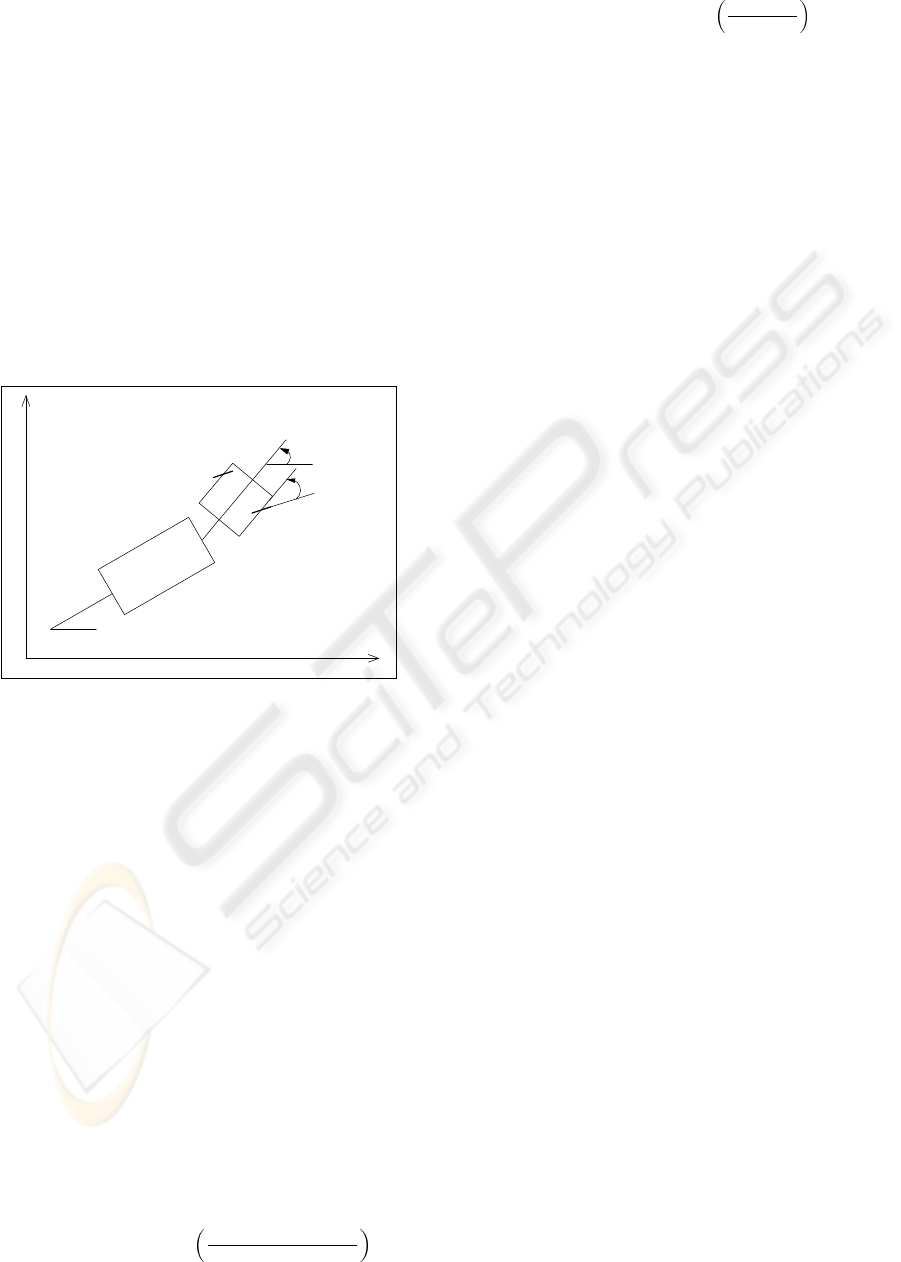
Figure 4: Truck and Trailer System Description.
Our model of the truck and trailer is based on the
set of equations presented in (Nguyen and Widrow,
1989). The system has four state variables, that
is the coordinates of the center rear of the trailer
(x, y ∈ [0, 50]), the angle of the trailer w.r.t. the x-
axis (θ
S
∈ [−90
◦
, 270
◦
]) and the angle of the cab
w.r.t the x-axis (θ
C
∈ [−90
◦
, 270
◦
]). We assume
that the truck moves backward with constant speed
of 2m/s, so the only control variable is the steering
angle u ∈ [−70
◦
, 70
◦
]. Fig. 4 shows a schematic view
of the truck and trailer system with its state and con-
trol variable. Moreover we single out 10 points in the
truck and trailer border (displayed in the Figure 4 by
bold points) representative of the truck and trailer po-
sition.
If the values of the state variables at time t are x[t],
y[t], θ
S
[t] and θ
C
[t], and the steering angle is u , then
the new values of state variables at time t + 1 are de-
termined by following equations:
x[t + 1] = x[t] − B ∗ cos(θ
S
[t]) (1)
y [t + 1] = y[t] − B ∗ sin(θ
S
[t]) (2)
θ
S
[t + 1] = θ
S
[t] − arcsin
A ∗ sin(θ
C
[t] − θ
S
[t])
L
S
(3)
θ
C
[t + 1] = θ
C
[t] + arcsin
r ∗ sin(u)
L
S
+ L
C
(4)
where A = r ∗ cos(u), B = A ∗ cos(θ
C
[t] −θ
S
[t]),
r = 1 is the truck movement length per time step,
L
S
= 4 and L
C
= 2 are the length of the trailer and
cab, respectively (all the measures are in meters).
After computing equations (3) and (4), the new
value of θ
C
is adjusted to respect the jackknife con-
straint: |θ
S
− θ
C
| ≤ 90
◦
.
Note that this model does not consider the obsta-
cles: indeed, embedding the obstacle avoidance in the
mathematical description of the truck and trailer dy-
namics would result in a untractable set of equations.
This feature will be added directly in the CGMurϕ
model described below.
5.2 The CGMurϕ Model
In the CGMurϕ model we use real values to repre-
sent the state variables x and y, whilst for the angle
values (i.e., θ
S
, θ
C
and u) it is sufficient, w.r.t. the
system dimensions, to use integer values. Moreover,
we define some tolerance constants to set up a range
of admissible final positions and angles for the center
rear of the trailer. These tolerances are used to define
the CGMurϕ goal property.
To embed the obstacles in the model, we approxi-
mate them through their bounding rectangles (or rec-
tangle compositions). Then we consider the repre-
sentative points of the truck-trailer position (defined
above, see Section 5.1) and, each time a new truck
position is computed, we use a function to check if
any of these points has hit the parking lot obstacles or
borders. Therefore, our controller synthesis algorithm
considers only feasible maneuvers to the goal state.
Moreover, in order to obtain a more robust con-
troller we also considered the maneuvering errors due
to the truck-trailer complex dynamic properties (e.g.,
friction, brakes response time, etc.) that cannot be
easily embedded in the mathematic model. We used
such errors to draw a security border around each ob-
stacle and used these augmented obstacles in the col-
lision check described above.
To estimate maximum maneuvering error we ap-
plied a Monte Carlo’s method described as follows.
We consider a large set of valid parking lot positions
S = {s
k
|1 ≤ k ≤ 500000}. Given a position s
k
∈ S,
(1) we apply a random maneuver m
k
obtaining the
new position ¯s
k
. Then (2) we randomly perturb s
k
generating the position s
p
k
and apply the same maneu-
ver m
k
on s
p
k
obtaining the position ¯s
p
k
. Finally, (3)
we compute the distance of the selected truck points
P
i
between the positions s
p
k
and ¯s
p
k
. This process is
repeated 200 times for each position in S, thus analyz-
ing 100 millions of perturbations. The security border
size is the highest distance measured for a point in the
step (3). We found out that this distance is 0.98m.
AUTOMATIC GENERATION OF OPTIMAL CONTROLLERS THROUGH MODEL CHECKING TECHNIQUES
31
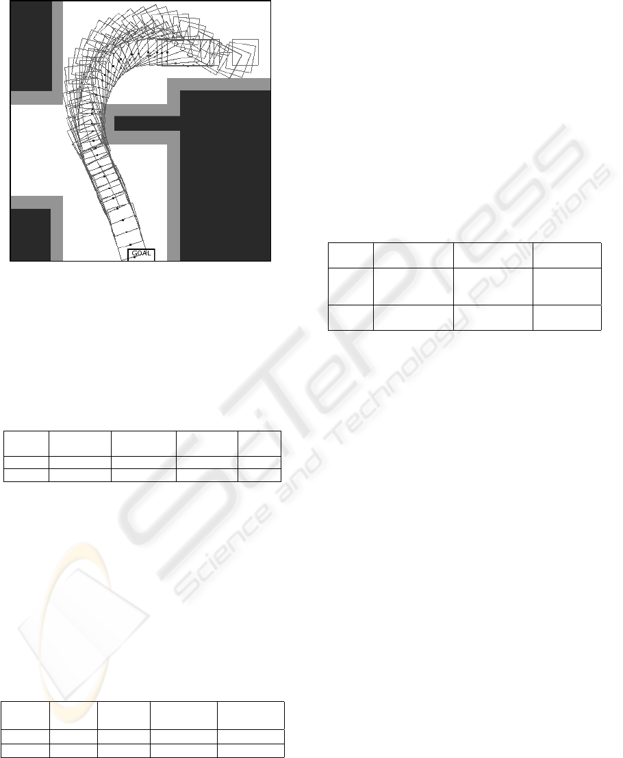
5.3 Experimental Results
Figure 5: Optimal trajectory generated by CGMurϕ from
initial position x = 12, y = 16, θ
s
= 0, θ
c
= 0.
We tested our methodology using several obstacles
topologies. In this section we present the results rel-
ative to the map shown in Fig. 5 where the obstacles
and the security borders are highlighted.
Table 1: Experimental results for optimal raw controller
synthesis.
Round Reachable Rules Trans. in Time
States Fired Controller Sec
0.5m 2233997 64785913 382262 8160
0.2m 12227989 354611681 1749586 32847
Table 1 shows the results of the first phase of our al-
gorithm (see Section 4.2). We repeated the controller
generation using two different approximations for the
real state variables x and y, rounding them to 0.5 and
0.2 meters.
Indeed, an higher precision extends the reachable
state space and, consequently, the number of transi-
tions in the controller. The results in Table 1 show
that we are able to deal with system having millions
of states.
Table 2: Experimental results for controller strengthening.
Round MAX Trans. Trans. in Size of
VARS Added Controller Controller
0.5m 36 257850 640112 14Mb
0.2m 36 646364 2395950 50Mb
In the second phase, we refined the controller by
applying 36 disturbs to each state in the controller ta-
ble and finding the appropriate rules to reconnect each
new state to the optimal controller paths, as described
in Section 4.3. As shown in Table 2, in this phase a
significant number of transitions is added, due to the
complexity of the truck-trailer dynamics.
5.3.1 Controller Robustness
In order to check the controller robustness, we consid-
ered all the trajectories starting from each state in the
controller. For each trajectory state s, we applied a
random disturbance on the state variables, generating
a possibly new state s
p
, and then we applied to s
p
the
rule associated to controller state s
′
that is nearest to
s
p
. A trajectory is robust if, applying the disturbances
above, it eventually reaches the goal state.
Table 3: Check of Controller Robustness.
Round Disturb Range Disturb Range Robust
for x,y for θ
s
,θ
c
Trajectories
0.5m ±0.25m ±1
◦
40%
±0.125m ±0.5
◦
45%
±0.0625m ±0.25
◦
57%
0.2m ±0.1m ±1
◦
74%
±0.05m ±0.5
◦
88%
We checked all trajectories by applying different
disturb ranges. As shown in Table 3, the fraction of
robust trajectories increases with the controller preci-
sion (i.e., the real values approximation). Note that
the percentages of robust trajectories in the second
round are completely satisfying considering:
• the optimality of the trajectories;
• the extreme complexity of this parking problem;
• the unavailability of correction maneuvers.
6 CONCLUSIONS
The controller tables generated through our method-
ology contain millions of state-rule pairs. Thus, if
we are working with small embedded systems, the ta-
ble size could be a potential issue. This problem can
be mitigated by applying various compression tech-
niques on the table.
A completely different solution that we are also ex-
perimenting is the generation of hybrid controllers,
that are optimal controllers working in parallel with
e.g. a fuzzy controller. In this case, the optimal con-
troller ensures the execution of the optimal plans (i.e.,
it is the optimal raw controller generated in Section
4.2), whereas the fuzzy controller is able to bring the
system back to the optimal plans from any state out-
side the optimal raw controller. Thus, the fuzzy con-
troller substitutes the extended knowledge generated
ICINCO 2006 - INTELLIGENT CONTROL SYSTEMS AND OPTIMIZATION
32

by the algorithm in Section 4.3 with a set of inference
rules. These rules may be in turn generated by an iter-
ative learning process driven by an algorithm similar
to the one of Section 4.3.
REFERENCES
˚
Astrom K.J, H. T. (2005). PID controllers - Theory, Design,
and Tuning. International Society for Measurement
and Con; 2nd edition.
Bertsekas, D. P. (2005). Dynamic Programming and Opti-
mal Control. Athena Scientific.
Burch, J. R., Clarke, E. M., McMillan, K. L., Dill, D. L.,
and Hwang, L. J. (1992). Symbolic model checking:
10
20
states and beyond. Inf. Comput., 98(2):142–170.
Cached Murphi Web Page (2006).
http://www.dsi.uniroma1.it/∼tronci/
cached.murphi.html.
Della Penna, G., Intrigila, B., Melatti, I., Tronci, E., and
Venturini Zilli, M. (2004). Exploiting transition local-
ity in automatic verification of finite state concurrent
systems. STTT, 6(4):320–341.
Dill, D. L., Drexler, A. J., Hu, A. J., and Yang, C. H. (1992).
Protocol verification as a hardware design aid. In Pro-
ceedings of the 1991 IEEE International Conference
on Computer Design on VLSI in Computer & Proces-
sors, pages 522–525. IEEE Computer Society.
Holzmann, G. J. (2003). The SPIN Model Checker.
Addison-Wesley.
Hu, A. J., York, G., and Dill, D. L. (1994). New tech-
niques for efficient verification with implicitly con-
joined bdds. In DAC ’94: Proceedings of the 31st
annual conference on Design automation, pages 276–
282, New York, NY, USA. ACM Press.
Jin, J. (2003). Advanced Fuzzy Systems Design and Appli-
cations. Physica-Verlag.
Kautz, H., Thomas, W., and Vardi, M. Y. (2006). 05241 ex-
ecutive summary – synthesis and planning. In Kautz,
H., Thomas, W., and Vardi, M. Y., editors, Synthe-
sis and Planning, number 05241 in Dagstuhl Seminar
Proceedings.
Li, H. and Gupta, M. (1995). Fuzzy Logic and Intelligent
Systems. Kluwer Academic Publishers.
Lygeros, J., Tomlin, C., and Sastry, S. (1999). Controllers
for reachability specifications for hybrid systems.
Murphi Web Page (2004). Murphi Web Page:
http://sprout.stanford.edu/dill/murphi.html.
Nguyen, D. and Widrow, B. (1989). The truck backer-
upper: an example of self learning in neural networks.
In In Proceeding of IJCNN., volume 2, pages 357–
363.
Sniedovich, M. (1992). Dynamic Programming. Marcel
Dekker.
Stern, U. and Dill, D. (1998). Using magnetic disk instead
of main memory in the murϕ verifier. In Hu, A. J. and
Vardi, M. Y., editors, Computer Aided Verification,
10th International Conference, CAV ’98, Vancouver,
BC, Canada, June 28 - July 2, 1998, Proceedings,
volume 1427 of Lecture Notes in Computer Science,
pages 172–183. Springer.
Stern, U. and Dill, D. L. (1995). Improved probabilis-
tic verification by hash compaction. In CHARME
’95: Proceedings of the IFIP WG 10.5 Advanced Re-
search Working Conference on Correct Hardware De-
sign and Verification Methods, pages 206–224, Lon-
don, UK. Springer-Verlag.
AUTOMATIC GENERATION OF OPTIMAL CONTROLLERS THROUGH MODEL CHECKING TECHNIQUES
33
