
A FUZZY APPROACH FOR FAULT DETECTION AND
ISOLATION OF UNCERTAIN PARAMETER SYSTEMS AND
COMPARISON TO BINARY LOGIC
Salma Bouslama Bouabdallah
Laboratoire Analyse et Commande des Systèmes (ACS), Ecole Nationale d’Ingénieurs de Tunis
B.P. : 37 - Le Belvédère – 1002 Tunis –Tunisie
Moncef Tagina
Ecole Nationale des Sciences de l’Informatique. Campus Universitaire – 2010 Manouba-Tunisie
Keywords: Fault Detection and Isolation, Bond Graph, Analytical Redundancy, uncertain parameter systems, Fuzzy
logic.
Abstract: This paper deals with fault detection and isolation off-line affecting sensors and actuators of uncertain
parameter systems modelled by bond graph. A fuzzy approach for fault detection based on residual
fuzzification is proposed. Besides, an isolation method based on fuzzy processing of the detection results is
proposed. Finally binary approach and fuzzy one are compared through an illustrative example.
1 INTRODUCTION
Due to the increasing size and complexity of modern
processes, their safety and their efficiency become
very important. The aim of our work is to keep
process in a good level of safety. Presently, fault
detection and isolation is an increasingly active
research domain. A process is in a defective state if
causal relations between its known variables
changed (Brunet J., 90). A widespread solution for
fault detection and isolation is to use analytical
model-based redundancy (Evsukoff A. et al., 2000).
The choice of a modelling formalism is an
important step for fault detection and isolation
because the quality of redundancy relations depends
on the quality of the model. In the frame of our work
we chose Bond graph modelling. In fact the Bond
graph is a powerful tool used for modelling the
dynamical systems. Thanks to its provided
information, bond graph can be used directly to
generate analytical redundancy relations between
known variables (Tagina M., 95).
Moreover, the system parameters are sometimes
uncertain; they can also be fluctuated by a wear, or
an external disturbance (Niesner C., 2004). Fuzzy
reasoning is a powerful tool for modelling the
uncertainty generated by models and sensor
imprecision as well as vagueness of the normal
behaviour limits (Evsukoff A. et al., 2000).
This paper proposes a fuzzy approach for fault
detection and isolation affecting sensors and
actuators of bond graph modelled uncertain
parameter systems.
In section 2, two methods for fault detection are
presented, one is based on a fixed threshold in order
to detect fault via a crisp decision, the other, which
is proposed, is based on fuzzification of residuals
provided by analytical redundancy relations (ARRs).
In section 3, an isolation method based on known
variables signature is presented, then an isolation
method based on fuzzy processing of the detection
results is proposed. Finally, in section 4, the classical
and the fuzzy approach are applied to an illustrative
example and results are compared in section 5.
98
Bouslama Bouabdallah S. and Tagina M. (2006).
A FUZZY APPROACH FOR FAULT DETECTION AND ISOLATION OF UNCERTAIN PARAMETER SYSTEMS AND COMPARISON TO BINARY LOGIC.
In Proceedings of the Third International Conference on Informatics in Control, Automation and Robotics, pages 98-106
DOI: 10.5220/0001217600980106
Copyright
c
SciTePress

2 FAULT DETECTION
METHODS FOR UNCERTAIN
PARAMETER SYSTEMS
2.1 Binary Logic Based Method
This technique consists on a test of the signal
amplitude. The adjustment parameters are the
thresholds regulated according to the various
operating assumptions and the desired performances
for detection (Brunet J., 90).
2.2 The Proposed Method Based on
Fuzzy Logic
Observed residuals, written in integral form obtained
when a rectangular fault affects sensors or actuators
in a limited interval, have the following forms:
(a)
(b)
0 1 2 3 4 5 6 7 8 9 10
-2.5
-2
-1.5
-1
-0.5
0
0.5
x 10
7
r3
temps
r3
data 1
(c)
Figure 1: Residual forms in case of a rectangular fault.
The (c) residuals can not be processed in the
same way as the (a) and (b) residuals. In fact for (a)
and (b) residuals, the fault cancellation brings back
the residual to a constant or null value. For the (c)
residual, the fault cancellation does not prevent its
divergence due to the double integration.
2.2.1 (a) and (b) Residuals
We have proposed in (Bouabdallah S. et al., 2005), a
fault detection method based on the fuzzification of
(a) and (b) residuals.
Fuzzy reasoning is composed of the following
stages: attribute fuzzification, application of
inference rules and defuzzification (Bûhler H., 94).
In the Fuzzy Logic Toolbox of Matlab 7.0, there
are five steps of the fuzzy inference process:
Step 1: Fuzzify inputs
It consists in taking inputs and determining the
degree to which they belong to each of the
appropriate fuzzy sets via membership functions. A
membership function is a curve that defines how
each point in the input space is mapped to a
membership value or degree of membership between
0 and 1. The output is then a fuzzy degree of
membership in the qualifying linguistic set.
Step 2: Apply Fuzzy Operator
Once the inputs have been fuzzified, we know the
degree to which each part of the antecedent has been
satisfied for each rule. If the antecedent of a given
rule has more than one part, the fuzzy operator is
applied to obtain one number that represents the
result of the antecedent for that rule. This number
will then be applied to the output function. The input
to the fuzzy operator is two or more membership
values from fuzzified input variables. The output is a
single truth value.
Step 3: Apply Implication method
Every rule has a weight (a number between 0 and 1),
which is applied to the number given by the
antecedent. Once proper weighting has been
assigned to each rule, the implication method is
implemented. A consequent is a fuzzy set
represented by a membership function, which
weights appropriately the linguistic characteristics
that are attributed to it. The consequent is reshaped
using a function associated with the antecedent (a
single number). The input for the implication
process is a single number given by the antecedent,
and the output is a fuzzy set. Implication is
implemented for each rule. Two built-in methods are
supported by fuzzy toolbox of Matlab 7.0, and they
are the same functions that are used by the AND
method: min (minimum), which truncates the output
fuzzy set, and prod (product), which scales the
output fuzzy set.
Step 4: Aggregate All Outputs.
Aggregation is the process by which the fuzzy sets
that represent the outputs of each rule are combined
into a single fuzzy set. The input of the aggregation
process is the list of truncated output functions
0
1
2
3
4
5
6
7
8
9
1
0
0
1
2
3
4
5
6
7
8
9
1
0
A FUZZY APPROACH FOR FAULT DETECTION AND ISOLATION OF UNCERTAIN PARAMETER SYSTEMS
AND COMPARISON TO BINARY LOGIC
99
returned by the implication process for each rule.
The output of the aggregation process is one fuzzy
set for each output variable.
Step 5 Defuzzify
The input for the defuzzification process is a fuzzy
set (the aggregate output fuzzy set) and the output is
a single number. There are five built-in
defuzzification methods supported by Fuzzy
Toolbox of Matlab 7.0: centroid, bisector, middle of
maximum (the average of the maximum value of the
output set), largest of maximum, and smallest of
maximum.
2.2.1.1 Fuzzification
Two set of features are used in the fuzzification
stage:
1. absolute value of the residual
provided by ARRs : r
2. variation |r-rfin| : d
With rfin is the final value of r.
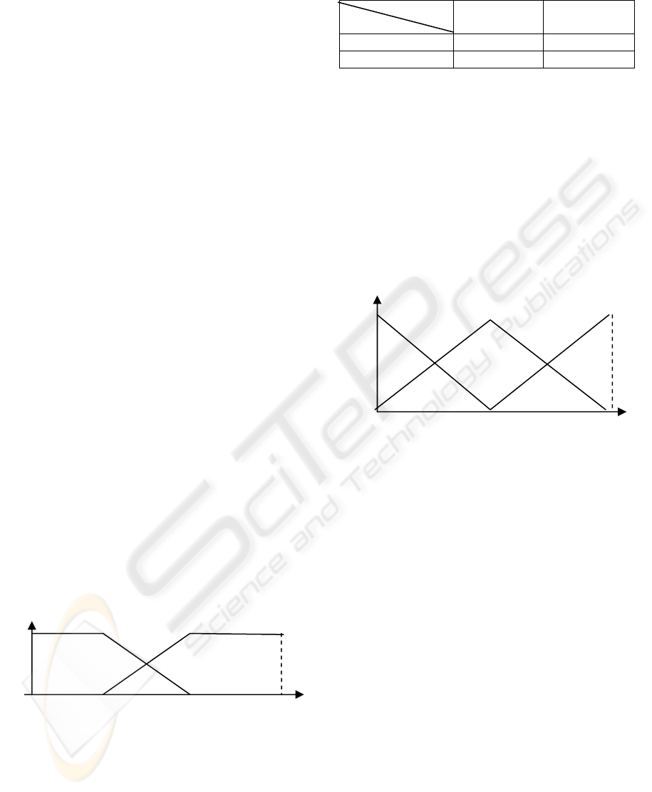
The linguistic set {small, large} is used to
describe the two attributes "r" and "d" which have
trapezoidal membership functions, the supports of
the membership functions are the same for "r" and
"d".
µ
Small
= [0, 0, r-max, Rmin ]
µ
Large
= [r-max, Rmin, Rmax, Rmax ]
with:
r-max: maximum value of r in fault free context.
Rmin: minimal value of r when a rectangular fault is
introduced in a limited interval.
Rmax: maximum value of r when a rectangular fault
is introduced in a limited interval.
Notice: r-max=d-max, Rmin=Dmin and
Rmax=Dmax.
Figure 2: Fuzzy Partition of r and d.
2.2.1.2 Inference Rules
We have established a set of inference rules which
are presented in the following table:
Table 1: Inference rules.
r
d
Small Large
Small Small Small
Large Small Large
We have used the method of inference max-min,
this method consists in using the operator min for
"AND" and the operator max for "OR".
2.2.1.3 Defuzzication
The defuzzification consists in transforming the
fuzzy information provided in the inference stage in
a real value. The output of the system is called Fault-
index.
Three membership classes of Fault-index are
defined: Small, Medium and Large.
Figure 3: Defuzzification of Fault-index.
The defuzzification provides a fault indicator, if
Fault-index is close to 0 it means that known
variables of the residual are in normal state. If Fault-
index is close to 1, that indicates the presence of a
fault. If Fault-index is in the interval [0.25 0.75],
then there is a detection problem.
2.2.2 (C) Residuals
It is assumed that, if a known variable appears in a
(c) residual, it appears also in (a) or (b) residuals.
We are interested now in a (c) residual rj, we
suppose that the system has m residuals (a) or (b)
having at least one common known variable with rj.
These residuals are r1, r2… rm.
The set of features of the system are: Fault-
index-1, Fault-index-2… Fault-index-m and rj
2.2.2.1 Fuzzification
The set {Small, Large} is used to describe all the
attributes of the system. For rj, we use the
membership functions presented in figure 2. For
µ
Small
µ
Large
1
0 0.25 0.5 0.75 1
µ Medium
µ
1
µ
Small
µ
Large
0
r
-max R
m
in Rmax
r
ICINCO 2006 - INTELLIGENT CONTROL SYSTEMS AND OPTIMIZATION
100

Fault-indexes, we use trapezoidal membership
functions. The supports of the membership functions
are as follows:
µ
Small
= [ 0, 0, 0.25, 0.75 ]
µ
Large
= [ 0.25, 0.75, 1, 1 ]
Figure 4: Fuzzification of Fault-index.
2.2.2.2 Inference Rules
The inference rules are based on the following
observation: the cancellation of a fault doesn’t
appear in a (c) residual because of its divergence,
(see figure 1).
The inference rules are as follows:
- IF rj is "Small" THEN Fault-index-j is "Small"
- IF rj is "Large" and Fault-index-i is "Large" THEN
Fault-index-j is "Large" (Fault-index-i is a fault
indicator of ri, 0<i<m+1)
- IF rj is "Large" and Fault-index-1 is "Small" and…
and Fault-index-m is "Small" THEN Fault-index-j is
"Small". ({Fault-index-1… Fault-index-m} is the set
of Fault-indexes corresponding to the residuals {r1,
r2… rm}).
2.2.2.3 Defuzzification
The defuzzification provides a fault indicator for the
residual rj. The output is called Fault-index-j. The
fuzzy partition of Fault-index-j is the same as the
fuzzy partition of Fault-index of (a) or (b) residuals.
3 FAULT ISOLATION
3.1 A Signature-based Isolation
Method
This method consists in associating each known
variable with a binary vector. The terms equal to 1
indicate the presence of the variable in the
corresponding residual. This binary vector is the
fault signature of the variable (
Tagina M., 95).
The residual processing provides a coherence
binary vector which terms equal to 1 indicate the
presence of a fault. For the fault isolation, the
coherence binary vector must be compared to the
various fault signatures as well as the normal
functioning mode signature.
3.2 The Proposed Fuzzy Isolation
Method
In this paragraph, we propose a fuzzy isolation
method. The attributes of the system are Fault-
indexes provided in the detection stage. The outputs
correspond to fault indicators of known variables
(Fault-j).
3.2.1 Fuzzification
The descriptive set {Small, Large} is used to
describe the Fault-indexes. The fuzzy partition is the
same as figure 4.
3.2.2 Inference Rules
We suppose that we have N residuals and M known
variables.
Fault signatures can be rewritten by replacing 1
by "Large" and 0 by "Small".
This allows writing inference rules in the form:
IF Fault-index-1 is ("Small"/"Large") and Fault-
index-2 is ("Small"/"Large")…and Fault-index-N is
("Small"/"Large") THEN Fault-j is
("Small"/"Large"), j ∈ {1, 2, ..,M}
Notice: Fault-j is "Large" in only one rule, this is
when the coherence binary vector is identical to fault
signature of the known variable j.
3.2.3 Defuzzification
Three membership classes of Fault-j are defined:
Small, Medium and Large.
Figure 5: Fault-j fuzzy partition.
The defuzzification provides a fault indicator in
known variable j (Fault-j), a value close to 0 means
that the variable j is in normal state, a value close to
µ
1
µ
Small
µ
Large
0 0.25 0.75 1
µ
Small
µ
Large
1
0
0.
2
5
0.5
0.75
1
µ Medium
A FUZZY APPROACH FOR FAULT DETECTION AND ISOLATION OF UNCERTAIN PARAMETER SYSTEMS
AND COMPARISON TO BINARY LOGIC
101
1 indicates the presence of a fault in variable j. If
Fault-j is in the interval [0,25 0,75], then there is an
isolation problem.
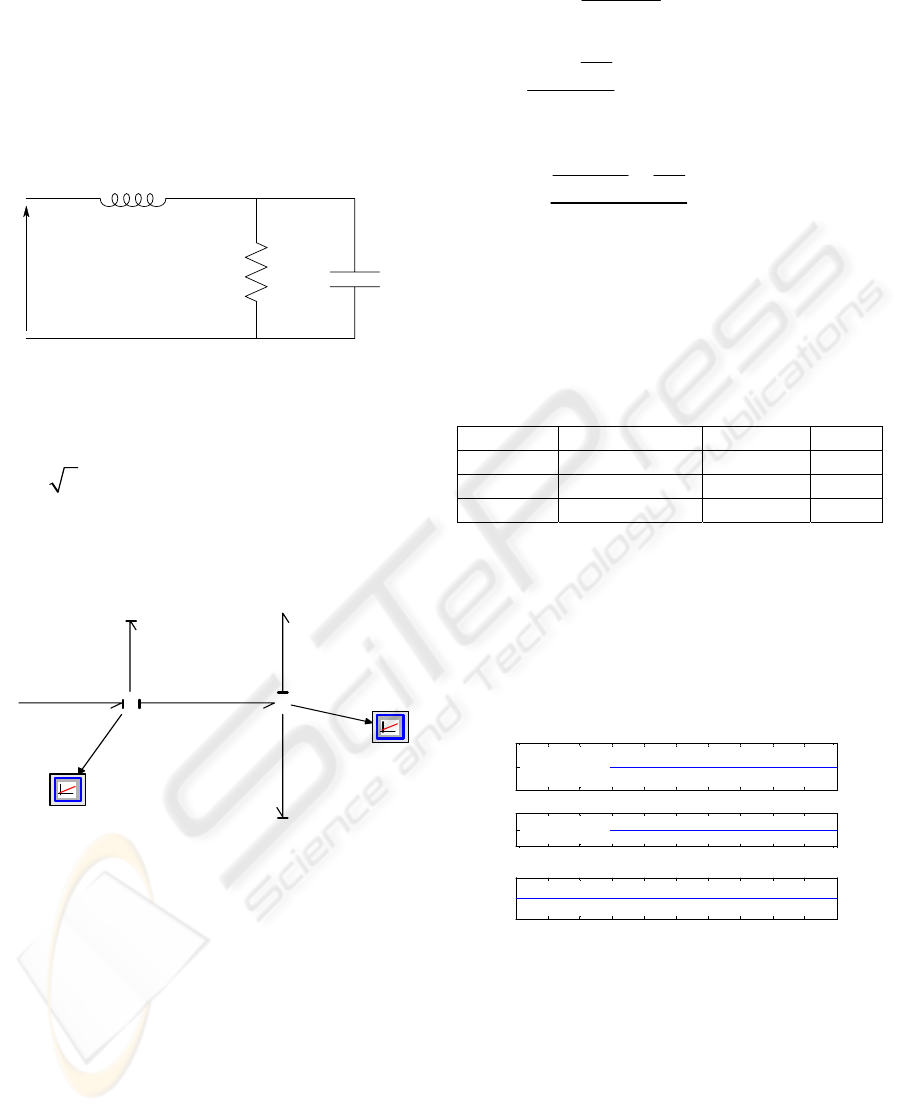
4 ILLUSTRATIVE EXAMPLE
We illustrate our approach with an RLC circuit:
Figure 6: RLC circuit in sinusoïdal mode.
With:
R = 500Ω, C = 5µF, L=0.2H, ω =1000 rd /s et
e(t) =
2 10sin (ωt ).
A procedure described in (Borne et al., 92) and
(Dauphin-Tanguy G. et al., 95) enables us to
elaborate its bond graph model shown in figure 7.
4
5
1
2
6
3
7
Se
e
1
O neJ unc tion1
0
Z eroJunc ti on1
I
L
C
C
R
R
Df
De
Figure 7: Bond graph model of the RLC circuit.
We have placed two sensors in the bond graph
model:
- An effort sensor De
- A flow sensor Df
Variables to be supervised (the known variables)
are De, Df and Se.
Analytical redundancy relations consist in
finding relations between known variables of the
system. We have elaborated the following analytical
redundancy relations (ARRs) from the bond graph
model by course of the causal paths. ARRs are
written in integral form.
RRA1 :
.
Se De
Df
Ls
−
= (1)
RRA2 :
0
.
De
Df
R
De
Cs
−
−
= (2)
RRA3 :
0
Se De De
Ls R
De
sC
−
−
−= (3)
The procedure of generating (ARRs) is described
in (
Tagina M.,95).
The fault signature table of the three known
variables (Se, De, Df) is given by table 2:
Table 2: Signature Table.
Se De Df
RRA1 1 1 1
RRA2 0 1 1
RRA3 1 1 0
The bond graph model is converted into a
synopsis diagram which is simulated under
Simulink/Matlab environment.
In normal functioning mode, the residuals have
to be close to zero. The simulation of the residuals
gives the following results:
0 1 2 3 4 5 6 7 8 9 10
-1
0
1
r1
0 1 2 3 4 5 6 7 8 9 10
-1
0
1
r2
temps
r2
0 1 2 3 4 5 6 7 8 9 10
-1
0
1
r3
temps
r3
Figure 8: residuals in fault free context and without
uncertainty in the components.
We verify that the three residuals are null.
Application choices:
* Uncertainty: We consider uncertainty as a white
noise added on R, L and C values in the synopsis
diagram (1% or 5% of each value). We have
selected uncertainty of 1% and 5% on one hand
because many components are given with this
uncertainty; on the other hand because the
L
e(t) R
C
ICINCO 2006 - INTELLIGENT CONTROL SYSTEMS AND OPTIMIZATION
102

identification is possible in this case. For larger
uncertainties, we can not distinguish between the
fault and uncertainty.
* Fault: We have considered fault as a rectangular
signal added to a known variable, the fault amplitude
is equal to 15% of the variables amplitude. We have
selected this amplitude because the noise-to-signal
ratio should not exceed 10%.
* Fault Interval length:
Faults are applied in intervals which length are
between 0.1s and 8s.
4.1 Case of 1% Uncertainty
The following results are obtained by simulation of
the three residuals r1, r2 and r3 in fault free context
and when faults are introduced in intervals which
lengths are between 0.1s and 8s:
Table 3: Characteristics for 1% of uncertainty.
r1-max 0.00188
R1min 0.0307
R1max 211.5
r2-max 0.0001615
R2min 0.001091
R2max 0.3
r3-max 19.62
R3min 1.232e+5
R3max 2.15e+8
We note that r1 and r2 are (a) and (b) residuals.
However r3 is a (c) residual.
A fault affects respectively Df, De and Se at time
4s up to 6s.
4.1.1 Fault Detection and Isolation by
Binary Logic
1
st
case: (a) and (b) residuals (r1 and r2)
The fault detection algorithm is as follows:
IF (ri > threshold-i and di >
threshold-i)
THEN Fault-index-i=1
ELSE Fault-index-i= 0
2
nd
case: (c) residuals (r3)
IF (r3 > threshold-3 and r2 <
threshold-2 and r1< threshold-1) or
(r3<threshold-3)
THEN Fault-index-3 = 0
ELSE Fault-index-3 = 1
The following thresholds are used in the
detection program: r-max, 2*r-max and Rmin.
We note that the fault detection is perfect for the
thresholds shown in table 4.
Table 4: Thresholds retained for 1% of uncertainty.
Residual Threshold
r1 2*r1-max
r2 r2-max
r3 2*r3-max
0 1 2 3 4 5 6 7 8 9 10
0
0.1
0.2
0.3
0.4
0.5
0.6
0.7
0.8
0.9
1
r1
temps (s)
Faul t-i ndex
Figure 9: (a) Fault-index-1, Fault index-2 and Fault-index-
3 when a fault affects De between 4s and 6s.
We can observe in figure 9 that Fault-index-1,
Fault-index-2 and Fault-index-3 are equal to 1 in the
interval where we have introduced the fault. This
lead to a coherence binary vector equal to [1 1 1] in
the interval [4s 6s], its comparison with different
signatures of table 2 locates the fault at the sensor
De.
We note that classical logic allows a perfect fault
detection and isolation if the threshold between
normal state and defective one is correctly chosen.
4.1.2 Fault Detection and Isolation by Fuzzy
Reasoning
By applying the proposed fuzzy approach to r1, r2
and r3 in Simulink/Matlab environment, we perform
good fault detection and isolation results for faults
affecting De, Se and Df.
Figure 10 shows detection when a fault affects
Df between 4s and 6s. Fault-index-1 and Fault-
index-2 are equal to 1 in this interval.
By applying the fuzzy isolation method (see
figure 11), we find that Fault-Df is equal to 1,
between 4s and 6s, whereas Fault-De and Fault-Se
are null in this interval, so we have perfectly isolated
fault at sensor Df.
A FUZZY APPROACH FOR FAULT DETECTION AND ISOLATION OF UNCERTAIN PARAMETER SYSTEMS
AND COMPARISON TO BINARY LOGIC
103

0 1 2 3 4 5 6 7 8 9 10
0
0.5
1
temps (s)
Fault-index-1
0 1 2 3 4 5 6 7 8 9 10
0
0.5
1
temps (s)
Fault-index-2
0 1 2 3 4 5 6 7 8 9 10
-1
0
1
temps (s)
Fault-i ndex-3
Figure 10: Fault-index-1, fault-index-2 and fault-index-3
when a fault affects Df.
0 1 2 3 4 5 6 7 8 9 10
0
0.5
1
temps (s)
Fault-Df
0 1 2 3 4 5 6 7 8 9 10
-1
0
1
temps (s)
Fault-De
0 1 2 3 4 5 6 7 8 9 10
-1
0
1
temps (s)
Fault-Se
Figure 11: Fault-Df, Fault-De and Fault-Se.
As a conclusion, in the case of 1% of
uncertainty, fuzzy approach as well as classical one
allows a good fault detection and isolation.
4.2 Case of 5% Uncertainty
The following results are obtained by simulation of
the three residuals r1, r2 and r3 in fault free context
and when faults are introduced in intervals which
lengths are between 0.1s and 8s.
Table 5: Characteristics for 5 % of uncertainty.
r1-max 0.009172
R1min 0.03643
R1max 215
r2-max 0.0008808
R2min 0.001092
R2max 0.3
r3-max 37.33
R3min 1.20e+5
R3max 2.16e+8
A fault affects respectively Df, De and Se at time
4s up to 6s.
4.2.1 Fault Detection and Isolation by
Binary Logic
We perform good fault detection and isolation
results for the following thresholds:
Table 6: Thresholds retained for 5% of uncertainty.
Residual Threshold
r1 2*r1-max
r2 r2-max
r3 2*r3-max
4.2.2 Fault Detection and Isolation by Fuzzy
Reasoning
In this case, we notice a small problem for faults
affecting Df. Figure 12 and figure 13 show that
Fault-index-1 and Fault-Df are disturbed in the
interval [4s 6s], however, we can isolate fault at
variable Df. Fault detection and isolation is good in
case of Se and De faults.
We conclude in the case of 5% uncertainty that
classical logic is more suitable for fault detection
and isolation.
0 1 2 3 4 5 6 7 8 9 10
0
0.5
1
temps (s)
Fault-index-1
0 1 2 3 4 5 6 7 8 9 10
0
0.5
1
temps (s)
Fault-index-2
0 1 2 3 4 5 6 7 8 9 10
-1
0
1
temps (s)
Fault-index-3
Figure 12: Detection: Fault-index-1, Fault-index-2 and
Fault-index-3 when a fault affects Df.
ICINCO 2006 - INTELLIGENT CONTROL SYSTEMS AND OPTIMIZATION
104

0 1 2 3 4 5 6 7 8 9 10
0
0.5
1
temps (s)
Fault-Df
0 1 2 3 4 5 6 7 8 9 10
-1
0
1
temps (s)
Fault-De
0 1 2 3 4 5 6 7 8 9 10
-1
0
1
temps (s)
Fault-Se
Figure 13: Isolation: Fault-Df, Fault-De and Fault-Se
When a fault affects Df.
4.3 Faulty Estimated Uncertainty
In practice, this case is very frequent, that is
generally due to a wear of components. Let us
consider the case where uncertainty reaches 5%
whereas the estimated one is equal to 1%.
4.3.1 Binary Logic
We apply the retained thresholds in case of 1%
uncertainty. As shown in figure 14, in the three cases
of faults, fault–index-1 is very disturbed, it passes
infinitely between 0 and 1outside the interval [4s
6s].
0 1 2 3 4 5 6 7 8 9 10
0
0.1
0.2
0.3
0.4
0.5
0.6
0.7
0.8
0.9
1
r1
temps (s)
fault-index-1
Figure 14: Fault-index-1 in all cases of faults.
So binary logic does not ensure good fault
detection in case of faulty estimated uncertainty.
4.3.2 Fuzzy Reasoning
By applying the fuzzy approach, the fault detection
and isolation is good for faults affecting De, Se and
Df. Figure 15 and figure 16 show fault detection and
isolation when a fault affects Df.
0 1 2 3 4 5 6 7 8 9 10
0
0.5
1
temps (s)
Fault-index-1
0 1 2 3 4 5 6 7 8 9 10
0
0.5
1
temps (s)
Fault-index-2
0 1 2 3 4 5 6 7 8 9 10
-1
0
1
temps (s)
Fault-index-3
Figure 15: Detection: Fault-index-1, fault-index-2 and
fault-index-3 when a fault affects Df.
0 1 2 3 4 5 6 7 8 9 10
0
0.5
1
temps (s)
Fault-Df
0 1 2 3 4 5 6 7 8 9 10
-1
0
1
temps (s)
Fault-De
0 1 2 3 4 5 6 7 8 9 10
-1
0
1
temps (s)
Fault-S e
Figure 16: Isolation: Fault-Df, Fault-De and Fault-Se in
case of a fault affecting Df.
5 COMPARISON
Binary logic allows performing good detection and
isolation results if the threshold is correctly chosen
and if the values of parametric uncertainty are
known. However, when uncertainty is faulty
A FUZZY APPROACH FOR FAULT DETECTION AND ISOLATION OF UNCERTAIN PARAMETER SYSTEMS
AND COMPARISON TO BINARY LOGIC
105

estimated, detection with binary logic is not suitable
whereas the fuzzy proposed approach allows
performing good fault detection and isolation results.
6 CONCLUSION
In this paper, we have proposed a fuzzy fault
detection and an isolation method for faults affecting
the sensors and the actuators off-line. A fuzzy
processing of residuals provided by ARRs is
followed by fuzzy processing of fault-indexes in
order to isolate the fault.
We have compared binary approach to fuzzy
approach through an illustrative example. We have
noticed that in the case of 1% or 5% of uncertainty,
binary logic allows a perfect fault detection and
isolation if the threshold between normal and faulty
state is correctly chosen, fuzzy approach allows also
fault detection and isolation in spite of some
disturbance in case of 5% uncertainty. However, in
case of faulty estimated uncertainty, the proposed
fuzzy approach allows good fault detection and
isolation where binary approach is not suitable for
fault detection and isolation.
REFERENCES
P. Borne, G. Dauphin-Tanguy, J. P. Richard, F. Rotella, I.
Zambettakis, « Modélisation et identification des
processus », Technip, 1992.
J. Brunet, « Détection et diagnostic de pannes approche
par modélisation », Editions Hermés, 1990.
S. Bouabdallah, M. Tagina, « Comparaison de la logique
classique et de la logique floue pour la détection des
défaillances des systèmes à paramètres incertains
modélisés par bond graph », STA’2005, Sousse,
Tunisie- pp. CM-35.
H. Bûhler, « Réglage par logique floue », Presses
polytechniques et universitaires Romandes, 1994.
G. Dauphin-Tanguy, «La méthodologie Bond graph
pour l’étude des systèmes physiques », Ecole de
printemps, Nabeul 1995, Tunisie.
Fuzzy logic toolbox. Matlab 7.0
A. Evsukoff, S. Gentil, J. Montmain, “Fuzzy reasoning in
co-operative supervision systems”, Control
Engineering Practice 8, 2000, pp. 389-407.
C. Niesner, G. Dauphin-Tanguy, « Sensibilité à
l’incertitude paramétrique - Une approche bond
graph », CIFA 2004, pp. 91-96.
M. Tagina, « Application de la modélisation bond graph à
la surveillance des systèmes complexes», Thèse de
doctorat 1995, Université Lille I, France.
S. Triki, M. Sayed Mouchaweh and B. Biera, « Méthode
de détection et d’aide à l’interprétation dans un
contexte de supervision », CIFA 2004, pp201-206
ICINCO 2006 - INTELLIGENT CONTROL SYSTEMS AND OPTIMIZATION
106
