
ACCURATE OBSERVER FOR MULTI-FAULT DETECTION AND
ISOLATION IN TIME VARYING SYSTEMS USING FAULT
CHARACTERIZATION
Ryadh Hadj Mokhneche and Hichem Maaref
Laboratoire Syst
`
emes Complexes
Universit
´
e d’Evry - CNRS FRE2494
40 rue du Pelvoux 91020 Evry, France
Keywords:
Multi-Fault Detection, Multi-Fault Observer, Fault isolation, Fault characterization, Time varying systems.
Abstract:
The usual observers up to now allowed the detection of faults in a parameter system via residue signals where
each one is judicious to detect one or more faults. However in the event of occurrence of several faults on the
same parameter, the residue signal of this observer will be able to detect them only if those are sufficiently
spaced intime. But in the event of their occurrence at very close moments, they will beoverlapped or compared
to only one fault and having a more significant amplitude. Thus, if a possible fault compensation is carried
out, it will be incorrect.
In this paper, it is proposed then an accurate observer for fault detection and isolation for one or several faults
on a same parameter and with a significant resolution. First, the characteristics of fault are shown to be used in
a goal of determinating the types of possible detections. An application of simulation is detailed and achieved
for fault detection in a sensor-based system, where the results are discussed. The succession effect of several
faults is tested, at one time or different times, on the amplitude, sign and general form of these faults. In the
end, the resolution of this observer is highlighted where a comparison between the usual observer and the
accurate observer is discussed.
1 INTRODUCTION
The problem of multi-fault detection in time variant
systems have always represented a subject of topical-
ity as studied in (V. Venkatasubramanian and Kavuri,
2003a), (V. Venkatasubramanian and Kavuri, 2003b),
(V. Venkatasubramanian and Yin, 2003), (P. Zhang
and Zhou, 2001), (R. Hadj Mokhneche and Vigneron,
2005), (Kuo and Golnaraghi, 2003) and (Rosenwasser
and Lampe, 2000).
Several works was completed during the two last
decades for only the fault detection problem in dy-
namical systems with simple or complex structure
(Gertler and Dekker, 2002), (A. Saberi and Niemann,
2000), that improve the importance of this problem
witch becomes increasingly current. The borders
between the various alternatives of approaches are
fuzzy; and some recent work showed that the ma-
jority of methods are closely related the ones to the
others (Kuo and Golnaraghi, 2003). There are sev-
eral approaches, methods and strategies for fault de-
tection and isolation, and the most used ones are
observer-based approaches (V. Venkatasubramanian
and Kavuri, 2003b).
Designing multi-fault detection system and its iso-
lation require a suitable compromise between raising
the sensitivity to faults and increasing the robustness
to unknown disturbances (Rosenwasser and Lampe,
2000). The most important part of model-based
approaches for multi-fault detection is the residual
generation problem and among the various existing
methods the most used are the observer-based plans
(Zhang, 2000) (Frisk and Nyberg, 2001). The signal
residue can detect more than one fault successively,
but if these faults occur at very close moments the ob-
server compares them to only one fault with charac-
teristics different that when these faults are detected
separately. Thus, it is proposed an accurate or pre-
cise observer which is able to detect these very close
faults without change on their amplitude and with a
significant resolution.
So, in what follows, the design of this accurate ob-
server is proceeded. Then, a complete simulation on
a system with speed observation is achieved. Several
comments and descriptions on this accurate observer
will be detailed. In the end, a general conclusion on
the results is given.
134
Hadj Mokhneche R. and Maaref H. (2006).
ACCURATE OBSERVER FOR MULTI-FAULT DETECTION AND ISOLATION IN TIME VARYING SYSTEMS USING FAULT CHARACTERIZATION.
In Proceedings of the Third International Conference on Informatics in Control, Automation and Robotics, pages 134-141
DOI: 10.5220/0001217201340141
Copyright
c
SciTePress
2 THE USUAL OBSERVER
It is described in order to determine the system dy-
namics integrating the observer. It will be explained
then its detection capacities limits.
2.1 Linear Case
Let us consider initially a dynamical system where
its state feedback control law is given by (Kuo and
Golnaraghi, 2003), (Rosenwasser and Lampe, 2000) :
u = −Kx (1)
u is the system command, K the gain matrix and x
the system state. Consider the system :
˙x = Ax + Bu
y = Cx
(2)
where y (t) is the output, C the application matrix of
state and where (A, C) is an observable pair. The ob-
server takes the form :
˙
ˆx = Aˆx + Bu
ˆy = C ˆx
(3)
By comparing the measured output with the output
computed from the state estimate, this gives
˜y = y − ˆy
= (Cx) − (C ˆx)
= C ˜x (4)
Computing the error dynamics once again, that
gives
˙
˜x = x −
˙
ˆx
= (Ax + Bu) − (A˜x + Bu + G (y − C ˆx))
= (A − GC) ˜x (5)
Then, the actual state dynamics become
˙x = Ax − BK ˆx
= Ax − BKx + BKx − BK ˆx
= (A − BK) x + BK (x − ˆx) (6)
As computed above, the state estimator error dy-
namics are
˙
˜x = (A − GC) ˜x (7)
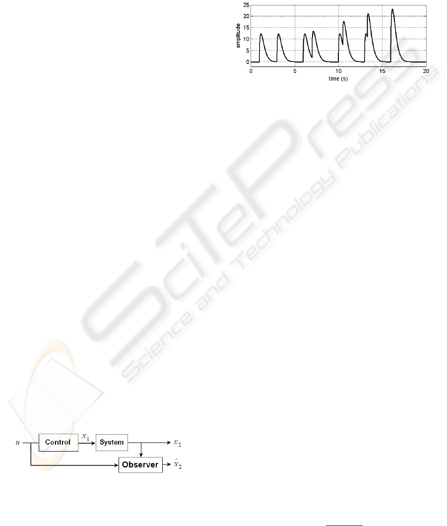
Figure 1: System connected to observer.
With such a dynamics and the observation system
showed on the figure (1), the observer generates the
signal r = ˆy − y (Kuo and Golnaraghi, 2003) which
is equal in this case to ˆx
2
− x
2
.
Example of this signal is shown by the figure (2)
where all faults have an amplitude value equal to 12.
Two faults are simulated at t = 16s but appear as one
fault with more significant amplitude, so the two fault
amplitudes are in pile up.
Figure 2: observer signal with multi-faults detection (linear
case).
2.2 Non-linear Case
One shall consider non-linear systems ((Jiang and
Chowdhury, 2004), (Tan and Edwards, 2003) and
(H. Hammouri and Yaagoubi, 1999)) of the form :
˙x (t) = f (x (t) , u (t)) ; x (0) = x
0
y (t) = Cx (t)
(8)
Proceeding by analogy to the classical observer de-
sign approach in the linear case, one seek an observer
of the following form :
˙
ˆx (t) = f (ˆx (t) , u (t)) + g (y (t)) − g (ˆy (t))
ˆy (t) = C ˆx (t)
with ˆx (0) = ˆx
0
(9)
The state and output errors are defined by :
e (t) = x (t) − ˆx (t)
ε (t) = y (t) − ˆy (t)
(10)
By omitting the time variable, the dynamic of esti-
mation error e(t) is then :
˙e = f (x, u) − f (ˆx, u) − g (y) + g (ˆy) (11)
Assuming that the observer state converges asymp-
totically to the state of the system, one can consider
the state error (equation 10) in the neighborhood of
zero. This allows the use of a first order Taylor ex-
pansion of the function f :
f (x, u) = f (ˆx + e, u) (12)
= f (ˆx, u) + D
ˆx
(f) e
where D
ˆx
; is a differential operator defined by :
D
ˆx
(f) =
∂f (x, u)
∂x
T
x=ˆx
(13)
ACCURATE OBSERVER FOR MULTI-FAULT DETECTION AND ISOLATION IN TIME VARYING SYSTEMS
USING FAULT CHARACTERIZATION
135
Similarly, for g :
g (y) = g (ˆy) + D
y
(g) Ce (14)
with :
D
y
(g) =
∂g (y)
∂y
T
y=ˆy
(15)
Consequently, the dynamic of the estimation error
may be rewritten :
˙e = [D
ˆx
(f) − D
y
(g) C] e (16)
A particular structure of the observer is proposed in
order to simplify the calculation of this mapping :
˙
ˆx (t) = f (ˆx, u) + R (ˆx, u) (y − ˆy)
ˆy = C ˆx
with ˆx (0) = ˆx
0
(17)
The state error is then solution of the equation :
˙e = f (x, u) − f (ˆx, u) − R (ˆx, u) (y − ˆy) (18)
The matricial function R(ˆx, u) is chosen so that
the state error e(t) asymptotically decreases and ap-
proaches zero as t tends to infinity. The error e(t) is
then considered to be in the neighborhood of zero. By
using (12) and (14), a first order Taylor expansion of
the function f(x, u) in the neighborhood of the esti-
mated state trajectory ˆx(t) is substituted in (18). that
gives :
˙e = [D
ˆx
(f) − R (ˆx, u) C] e (19)
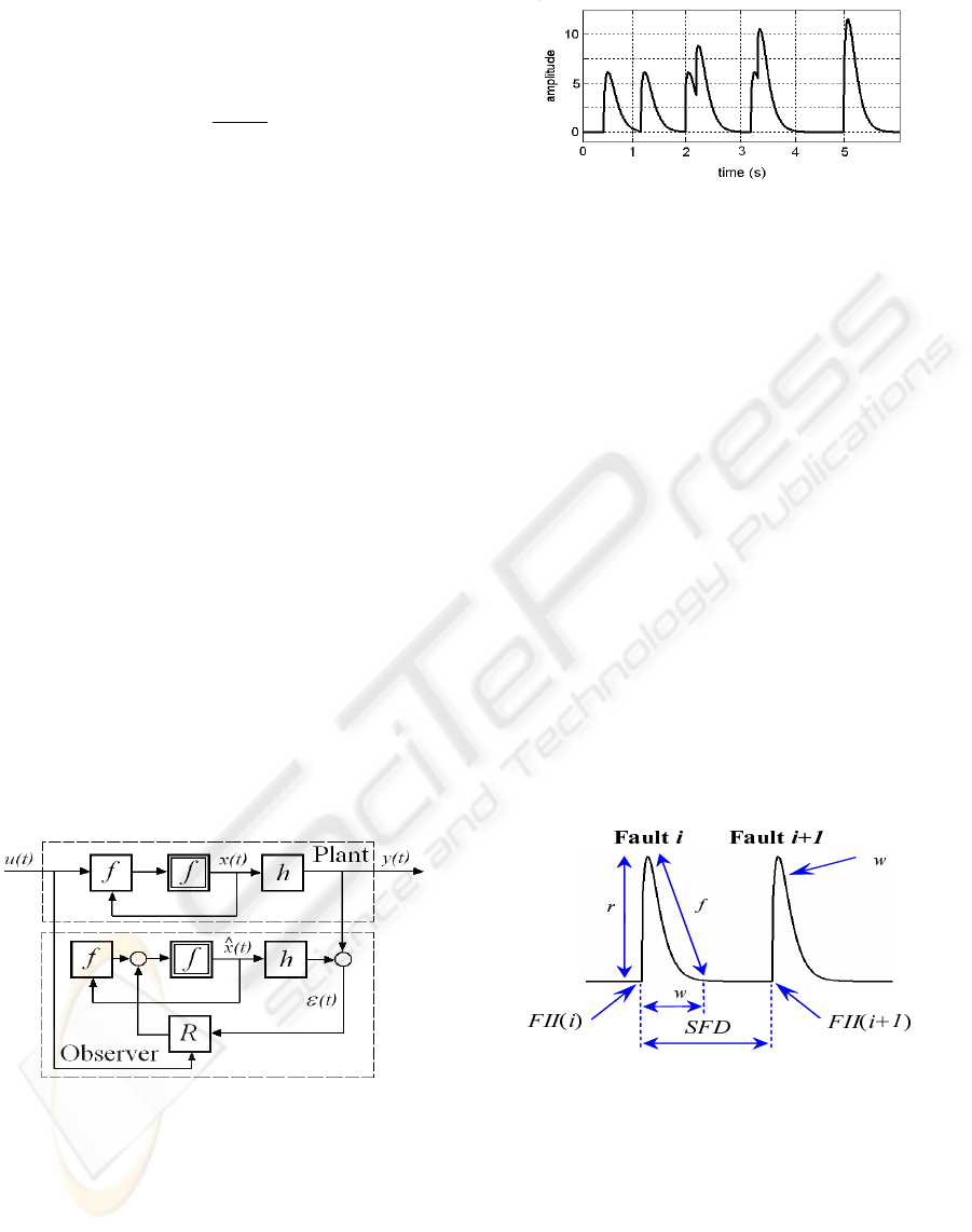
The block diagram of the resulting non-linear ob-
server is shown in figure 3 where the time invariant
matrix R(ˆx, u) has to be determined using the algo-
rithm obtained by the derivate of the quadratic Lya-
punov function (K. Adjallah and Ragot, 1994).
Figure 3: Non-linear observer.
With the observation system showed on figure (3),
the observer generates the residual signal shown on
figure (4), in absence of noise, where all faults have an
amplitude value equal to 7. Two faults are simulated
at t = 5s but appear as one fault with more significant
amplitude, so the two fault amplitudes are in pile up..
It will be further shown (section 5) that this usual
observer provides residue signals limited in precision
Figure 4: observer signal with multi-faults detection (non
linear case).
and that it can not detect two or several very close suc-
cessive faults (figures 2 and 4) beyond a certain limit
which will be defined. Moreover, the amplitudes of
the very close faults pile up to form only one fault,
which makes incorrect detection. In what follows,
a precise observer is carried out and which makes it
possible to cure these problems and which has signif-
icant characteristics.
3 ACCURATE OBSERVER
When a system parameter undergoes more than one
fault at very close moments, the usual observer assim-
ilates all the faults to only one fault with more impor-
tant amplitude in residue signal. A precise observer
must be able to detect them clearly and separately, so
to have a high resolution of detection. This leads us to
define the types of detection being able to take place
during a multi-fault detection.
f
d
t
t
Figure 5: Residue signal with two completely detected
faults.
3.1 Types of Detection
Consider the residue signal represented by the figure
(5) where the Successive Fault Duration SF D is the
duration between two successive completely faults,
d
w
(wrap duration) = F ID (Fault Incidence Dura-
tion) is the duration running out between the fault in-
ICINCO 2006 - SIGNAL PROCESSING, SYSTEMS MODELING AND CONTROL
136
cidence instant F II of fault i and the instant when the
residue takes the first value zero or close to zero. t
r
and t
f
are successively raising time and failing time
of the complete fault wrap f
w
.
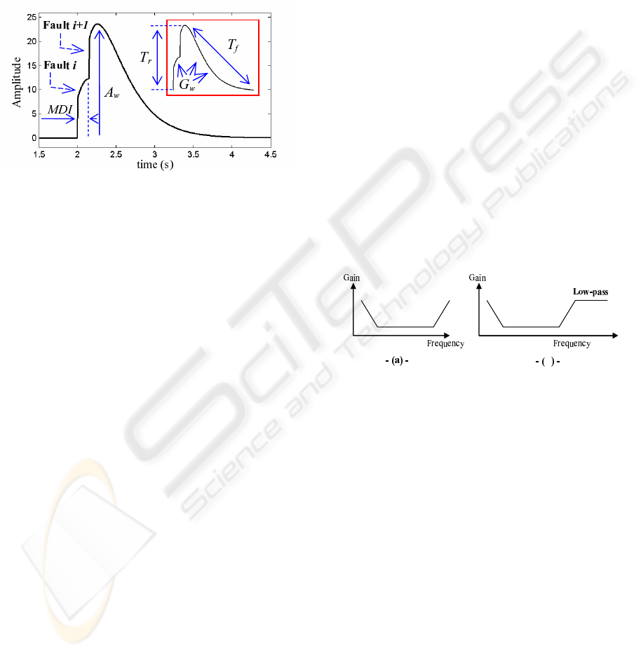
Consider also the figure (6) where M DI is the min-
imum duration of incidence corresponding to duration
between the F II(i) and the finish of the raising time
t
r
of fault i.
Figure 6: Residue signal with two skewed detected faults.
Three types of two-successive-fault detection can
be distinguished :
3.1.1 Complete Fault Detection
In this kind of detection, the two faults are completely
detected, i.e. SF D ≥ F ID (figure 5).
3.1.2 Partial Fault Detection
That means that it satisfied M DI < SF D < F ID
(figures 5 and 6). The fault i + 1 occurs during the
failing time t
f
of fault i, so The fault i is partially de-
tected. The amplitude of fault i + 1 take a more sig-
nificant value than envisaged and not representative,
what will generate an incorrect eventual compensa-
tion for this usual observer.
3.1.3 Skewed Fault Detection
It is obtained where SF D ≤ M DI (figure 6). The
fault i + 1 occurs during the raising time t
r
of fault i.
There is impression thus to detect only one fault and
the amplitude corresponds to the pile up of the two
faults amplitude. Also, the two faults raising time,
successively failing time, pile up to give a total raising
time T
r
, successively failing time T
f
. The two faults
wrap are rides and take then a global wrap G
w
. This
type of detection with usual observer will lead to an
incorrect eventual compensation.
3.2 Accurate Observer for
Multi-fault Detection
To solve the problems above, it is proposed an ac-
curate observer which uses a modified PID filter and
allows the detection of all secondary faults even those
occurring during the raising time of the current fault.
The behavior of PID filter can be characterized in
terms of its frequency response. A typical curve, as
shown in figure (7a), reveals distinct segments named
PID elements, each correlating to a different PID
term. The damping operation, KD, is a high pass filter
with gain that keeps increasing with frequency. This
is due to the nature of the derivative function. The
effect of increased gain is highly undesirable in sys-
tems with noise. In fact, all high frequency noise gets
amplified by the KD filter element, further intensify-
ing its damaging effect. This problem can be solved
by modifying the PID filter such that the gain curve
levels off beyond a given frequency (figure 7b). So,
the high frequency gain is limited to a fixed value,
thereby reducing the effect of the noise. The gain
limit is produced by a low pass filter. The modified
compensation technique essentially amounts to a PID
filter followed by a low-pass filter.
KI
KD
KP
KI
KD
KP
b
Figure 7: The frequency response of a PID filter (a) and of
a low pass filter added to PID filter (b).
With using modified PID filter as explained previ-
ously, the noise in the residue will considerably be re-
duced and the amplitude of residue could be limited.
Thus that leads us to obtain a robust observer to noise.
The modified PID filter associated to observer give us
the accurate observer.
4 APPLICATION
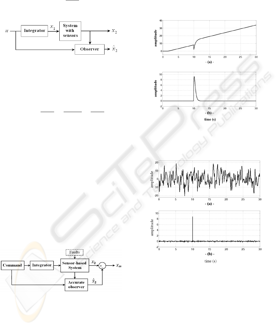
4.1 Presentation
The figure (8) represents a system to observing speed
where the system is a sensor-based one. x
1
and x
2
are
state variables and x
1
the speed to observe. The ob-
server is designed to follow x
1
by knowing the signals
x
2
and u.
ACCURATE OBSERVER FOR MULTI-FAULT DETECTION AND ISOLATION IN TIME VARYING SYSTEMS
USING FAULT CHARACTERIZATION
137
Here, the signal x
2
is obtained starting from the
signal x
1
using a sensor with transfer function H(s) :
H (s) =
2 − s
2 + s
(20)
where s is a symbolic parameter.
Figure 8: System connected to observer.
The associated equation to integrator block is ˙x
1
=
u. The transfer function of sensor block decay in the
following form
H (s) =
2 − s
2 + s
=
−s − 2
s + 2
+
4
s + 2
(21)
which a realization of state is
˙x
c
= −2x
c
+ x
1
x
2
= 4x
c
− x
1
(22)
where x
c
is intermediate characteristic variable.
The states of the observer to synthesize are ˆx
1
and
ˆx
2
which follow the states x
1
and x
2
respectively.
After transformations and calculations, an asymptotic
observer is looked for by considering the error predic-
tion which is here the considered residue :
r = ˆy − y = ˆx
2
− x
2
(23)
5 TESTS AND RESULTS
The diagram of figure (9) shows the simulation
scheme of one or several faults (external disturbances)
applied to the sensor-based system.
Figure 9: multi-fault system with the observer.
An observer is designed and set to estimate the out-
put signal of the system. It enables us to deduce the
predictive error and thus the residue signal x
r
of the
usual observer and the residue signal x
m
of the accu-
rate observer whose PID parameters are judiciously
calculated. Simulation is achieved in the single fault
case and in the the two or several faults case.
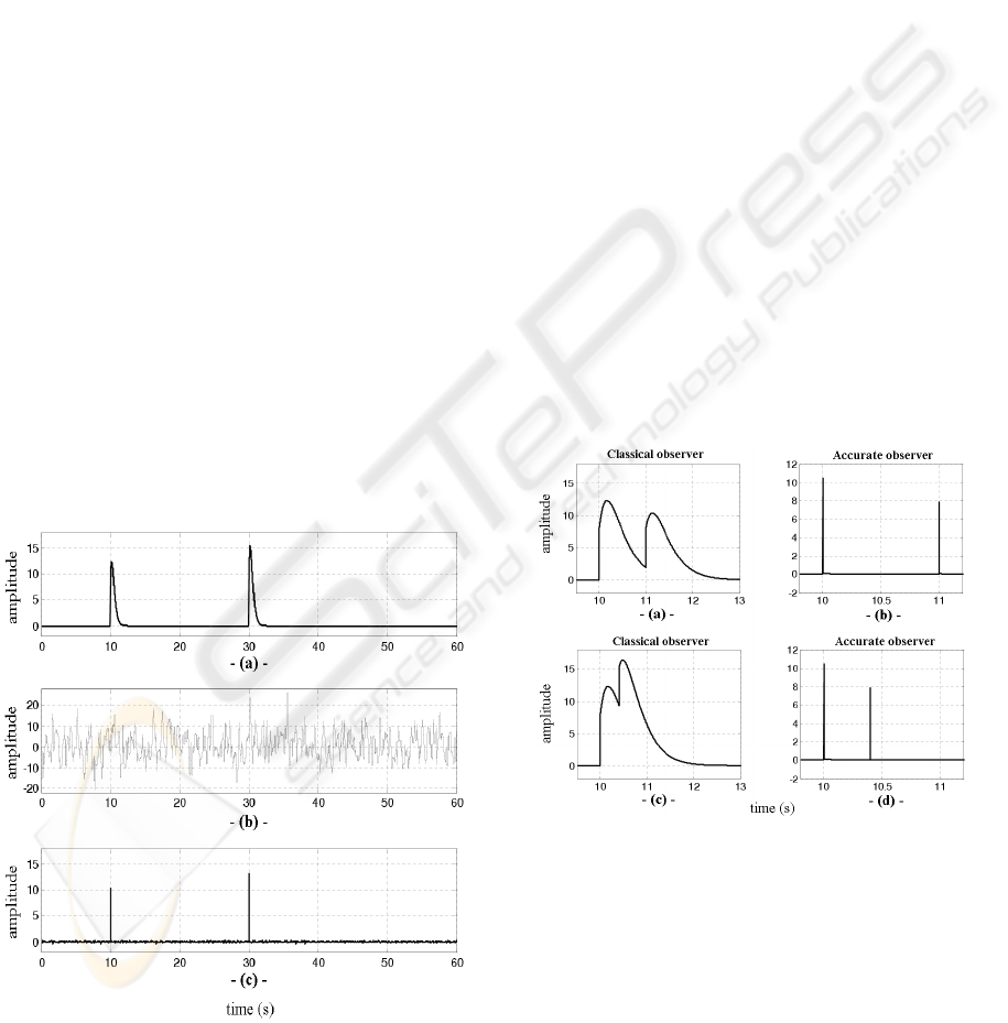
5.1 Single Fault Case
A fault is simulated at t = 10s, its effect is visible in
sensor signal (fig. 10a) and residue signal (fig. 11).
Figure 10: usual observer : Noiseless sensor signal x
2
(a)
and noiseless residue signal x
r
(b).
Figure 11: Residue signal in presence of noise : usual ob-
server (a) and accurate observer(b).
In absence of noise : When there are no faults, the
residue r tends to zero as ensured by the convergence
of the observer. Thus after the transient of the ob-
server, and before the incident of fault, it can be con-
sidered that the residue is practically zero. The occur-
rence of a fault modifies the behavior of the residue
signal as shown on figure (10b).
Let us suppose that the fault corresponds to a
change in one parameter of the sensor. As the
observer generating x
r
still relies on the nominal
ICINCO 2006 - SIGNAL PROCESSING, SYSTEMS MODELING AND CONTROL
138
parameter value, x
r
will not remain zero. After a
transient of the observer, the residue x
r
tends back to
zero, as the new value of the estimate parameter is
being correctly estimated by the observer. It should
be noted that signal x
m
is identical to that of x
r
except that duration F ID = d
w
(see figure 5) is very
close to zero.
In presence of noise : Now it is assumed that
the output measurement x
2
is noise corrupted. If
the noise is small compared to the effect of fault on
the residue, then the fault detection can still reason-
ably be performed through visual inspection of the
residue. However, if the noise is relatively high, then
the change in the behavior of the residue after the oc-
currence of a fault will be more or less hidden by the
noise. The figure (11a) shows the residue signal of
noise corrupted usual observer where the fault does
not appear.
The figure (11b) shows the signal x
m
of noise cor-
rupted accurate observer where the fault is clearly de-
tected with an F ID close to zero.
5.2 Two or Several Faults Case
5.2.1 Detection of Distinguished Faults
Initially four faults are simulated, two same faults at
the same moment t = 10s and two same others at the
same moment t = 30s (figure 12).
Figure 12: Residue signal in presence of 4 faults (two added
by two) : noiseless (a) and noise corrupted (b) usual ob-
server, noise corrupted accurate observer (c).
One remarks that in noiseless usual observer case,
the amplitudes of the faults inflicted in the same in-
stant appear in the residue while accumulating in
pile-up and thus the total amplitude of the residue
increased (figure 12a). The figure (12b) shows the
noise corrupted usual observer where faults are not
detected. In noise corrupted accurate observer case,
the faults are clearly detected although there is an in-
crease on amplitude (figure 12c).
While comparing the residue amplitude at instant
t = 10s to that at t = 30s of figure (12), the residue
amplitude is independent of the occurring moment of
fault.
5.2.2 Not Distinguished Faults
For the type of partial detection (figure 13) it was sim-
ulated two faults, one at the instant t = 10s with am-
plitude 12 and the other at the instant t = 11s with
amplitude 8.
One can remark that in usual observer case, as far
as the second fault is close to the first (figures 13a
and 13c), i.e. that F ID decreases until reaching the
maximum of first fault amplitude, the amplitude of
the second fault increases and tends to hide the first
one.
Figure 13: Noiseless residue signals in presence of two
faults at very close moments corresponding to partial de-
tection (M DI < SF D < F I D).
But in the accurate observer case (figures 13b and
13d), the faults are clearly apparent with their exact
amplitudes.
Detections seeming like impulses at the instants
10s and 11s (figure 13b) and at the instants 10s and
10.4s (figure 13d), and of all simulations in the accu-
rate observer case, are made up each one of a raising
ACCURATE OBSERVER FOR MULTI-FAULT DETECTION AND ISOLATION IN TIME VARYING SYSTEMS
USING FAULT CHARACTERIZATION
139
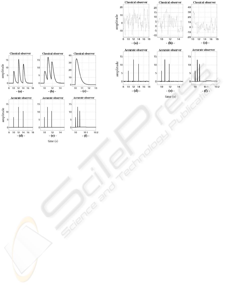
time and a failing time like those represented on the
figures (13g) and (13h).
The simulations of figures (14) and (15) are
achieved with tree faults at instant t = 10s, 12s and
14s, with amplitudes respectively 7, 15 and 12, in ab-
sence of noise. They summarize the three types of
detection described in paragraph (3.1), respectively in
absence and in presence of noise.
Figure 14: The three types of detection - presence of tree
faults at very close moments : Noiseless case.
The figures (14a) and (14b) showed respectively
the complete detection with usual observer and with
accurate observer, where the three faults are clearly
detected with exact amplitudes. For the partial fault
detection, the simulation is shown on figures (14b)
and (14e) where the usual observer detects partially
the second and third faults and with an increase in the
amplitude, but the accurate observer detects clearly
the tree faults and without increase in the amplitude.
In case of skewed detection (figures 14c and 14f), the
usual observer detects the faults but assimilates them
to only one fault instead of three and with a big in-
crease in the amplitude (pile up of the amplitudes of
the three faults). The accurate observer detect them
all and clearly.
The noise corrupted case for the three types of fault
detection is shown on figure (15) and where, in oppo-
site of usual observer, the faults are clearly detected
by the accurate observer.
5.3 Observer Resolution
5.3.1 Usual Observer
The limit capacity of usual observer to detect two suc-
cessive faults in absence of noise is shown on figure
Figure 15: The three types of detection - presence of tree
faults at very close moments : Noise corrupted case.
(16a) for the limit skewed detection case (SF D =
MDI). On figure (16c), for the skewed detection
case (SF D < MDI), one can remark that there is
an impression that it was detected only one fault. In
noise corrupted case, there is not faults detected (fig-
ures 16b and 16d). One is interested rather in the com-
pletely detected faults, thus to F ID. This last one is
in this usual observer case equal to 2s which is enor-
mous. So, if faults occur with SF D < 2s then they
will not be correctly detected or not a whole detected.
5.3.2 Accurate Observer
The figures (16g) and (16h) shows the effectiveness
of the accurate observer to detect two faults with sig-
nificant resolution in absence of noise (16g) and in
presence of this one (16h). This is valid also for sev-
eral faults. The resolution of this observer, with step
size simulation fixed above, is F ID = 0.002s which
is twice of step size.
The figures (16e) and (16f) show simulations done
respectively in absence and in presence of noise with
(SF D = M DI) where the M DI reached and cor-
responding to this limit is 0.2s. So that, the accurate
observer can detect faults occurring with SF D less
than the F ID of usual observer. The F ID founded,
corresponding to the limit complete detection of ac-
curate observer is 0.002s. One can easily remark that
this resolution is very precise compared to limit of
that from usual observer where the F ID is 0.2s (fig-
ure 14a).
ICINCO 2006 - SIGNAL PROCESSING, SYSTEMS MODELING AND CONTROL
140
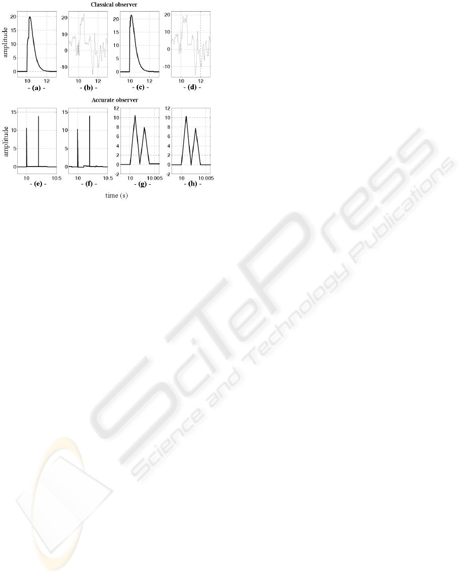
Figure 16: Resolution of the observer in the noiseless and
noise corrupted cases.
6 CONCLUSION
It was highlighted, using fault characterization, the
detection of several successive faults at same mo-
ments and at different moments. It was proved that
the moment of fault incidence does not affect the cor-
responding residue amplitude and it was seen that the
observer follows well the sign of the fault. It was pro-
ceeded a detection of several successive faults with
very close moments, in absence and in presence of
noise, corresponding to a resolution with an F ID
equal to twice of simulation step size. The ampli-
tudes of the faults were respected, thus avoiding the
pile up effect due before to the SF D durations which
were lower than M DI durations. The signs of the
faults amplitudes were also respected, thus allowing
a correct eventual future compensation by taking into
account the sign of the residue signal.
Three important characteristics of this accurate ob-
server can be noted. The first one is its robustness
to noise as shown in different preceding simulations,
the second one concern the amplitudes where are con-
served and the third one is the resolution where sev-
eral faults occurring in very close instants are clearly
detected. Comparing F ID of the usual observer to
that of the accurate observer, the second one can de-
tect a significant number of complete faults.
An other interesting characteristic is about the rais-
ing and failing times which are very short and right
which implies that the accurate observer has signifi-
cant resolution.
REFERENCES
A. Saberi, A. A. Stoorvogel, P. S. and Niemann, H. (2000).
Fundamental problems in fault detection and identifi-
cation. International Journal of Robust and Nonlinear
Control, 10:1209–1236.
Frisk, E. and Nyberg, M. (2001). A minimal polynomial
basis solution to residual generation for faultdiagnosis
in linear systems. Automatica, 37:1417–1424.
Gertler, J. J. and Dekker, M. (2002). Fault detection and di-
agnosis in engineering systems. Control Engineering
Practice, 10:1037–1040.
H. Hammouri, M. K. and Yaagoubi, E. H. E. (1999).
Observer-based approach to fault detection and iso-
lation for nonlinear systems. IEEE Transactions on
Automatic Control, 44:1879–1884.
Jiang, B. and Chowdhury, F. (2004). Observer-based fault
diagnosis for a class of nonlinear systems. Proceed-
ing of the 2004 American Control Conference, Boston,
Massachusetts, USA, 6:5671–5675.
K. Adjallah, D. M. and Ragot, J. (1994). Non-linear
observer-based fault detection. Proceedings of the 3rd
IEEE Conference on Control Applications, 2:1115–
1120.
Kuo, B. C. and Golnaraghi, F. (2003). Automatic control
systems, 8th edition. Eds John Wiley and Sons, New
York.
P. Zhang, S. X. Ding, G. Z. W. and Zhou, D. H. (2001).
An fdi approach for sampled-data systems. the 2001
American control conference, Arlington, USA, pages
2702–2707.
R. Hadj Mokhneche, H. M. and Vigneron, V. (2005). Hy-
brid algorithms for the parameter estimate using fault
detection, and reaching capacities. The 2nd Interna-
tional Conference on Informatics in Control, Automa-
tion and Robotics ICINCO, Barcelona, Spain, 4:289–
293.
Rosenwasser, E. N. and Lampe, B. P. (2000). Computer
controlled systems: analysis and design with process-
orientated models. Communications and Control En-
gineering, Eds. Springer, London, UK.
Tan, C. P. and Edwards, C. (2003). Sliding mode observers
for robust detection and reconstruction of actuator and
sensor faults. International Journal of Robust and
Nonlinear Control, 13:443–463.
V. Venkatasubramanian, R. Rengaswamy, K. Y. and Kavuri,
S. N. (2003a). A review of process fault detection and
diagnosis. part i: Quantitative model-based methods.
Computers and Chemical Engineering, 27:293–311.
V. Venkatasubramanian, R. R. and Kavuri, S. N. (2003b). A
review of process fault detection and diagnosis. part ii:
Qualitative models and search strategies. Computers
and Chemical Engineering, 27:313–326.
V. Venkatasubramanian, R. Rengaswamy, S. N. K. and Yin,
K. (2003). A review of process fault detection and di-
agnosis. part iii: Process history based methods. Com-
puters and Chemical Engineering, 27:327–346.
Zhang, Q. (2000). A new residual generation and evalu-
ation method for detection and isolation of faults in
non-linear systems. International Journal of Adaptive
Control and Signal processing, 14:759–773.
ACCURATE OBSERVER FOR MULTI-FAULT DETECTION AND ISOLATION IN TIME VARYING SYSTEMS
USING FAULT CHARACTERIZATION
141
