
DYNAMIC GOAL COORDINATION IN PHYSICAL AGENTS
Jose Antonio Martin H.
Faculty of Computer Science, Universidad Complutense de Madrid
C. Prof. Jos
´
e Garc
´
ıa Santesmases, 28040, Cuidad Univesitaria, Madrid, Spain
Javier de Lope
Dept. Applied Intelligent Systems, Universidad Polit
´
ecnica de Madrid
Campus Sur, Ctra. Valencia, km. 7, 28031 Madrid, Spain
Keywords:
Dynamic Optimization, Goal Coordination, Robotics, Multi-Objective Optimization, Reinforcement Learn-
ing, Optimal Control.
Abstract:
A general framework for the problem of coordination of multiple competing goals in dynamic environments
for physical agents is presented. This approach to goal coordination is a novel tool to incorporate a deep co-
ordination ability to pure reactive agents. The framework is based on the notion of multi-objective optimiza-
tion. We propose a kind of “aggregating functions” formulation with the particularity that the aggregation is
weighted by means of a dynamic weighting unitary vector
−→
ω (S) which is dependant on the system dynamic
state allowing the agent to dynamically coordinate the priorities of its single goals. This dynamic weighting
unitary vector is represented as a set of n − 1 angles. The dynamic coordination must be established by means
of a mapping between the state of the agent’s environment S to the set of angles Φ
i
(S) using any sort of
machine learning tool. In this work we investigate the use of Reinforcement Learning as a first approach to
learn that mapping.
1 INTRODUCTION
The problem of designing controllers for physical
agents (i.e. robots) is a very active area of research.
Since its early beginnings in the middle of the past
century many different approaches have been pro-
posed. The control paradigms where changing grad-
ually from the deliberative paradigm to the reactive
paradigm and from pure mathematical and engineer-
ing formulation to more biological formulations, ap-
proximating very different fields of research. One of
the fruitful branches of study has come to be called
the bio-inspired paradigm or bio-mimetic approach
(Passino, 2005).
In this paper we formulate a bio-inspired approach
to solve the problem of multiple goal coordination
for physical agents in dynamic environments. This
problem is the task to assign the right priority to
each agent’s goal leading to the design controllers fol-
lowing a pure reactive approach. Pure reactive ap-
proaches have been applied successfully to tasks like
robot navigation with collision avoidance. Despite
that, there are more complicated tasks where a single
reactive behavior is not enough. Such kind of tasks
involve multiple goals where the agent needs to bal-
ance the importance of each particular goal. The most
difficult problem from this point of view is when mul-
tiple goals are in conflict (competing goals), that is,
by following a pure reactive behavior the direct at-
tainment of one goal results in a loss in the attainment
of another goal. This situation is very common in real
tasks like collision avoidance vs. goal reaching and
pursuit and evasion games.
In order to deal with this kind of problem still fol-
lowing a reactive bio-inspired approach we have de-
veloped a framework for the dynamic goal coordina-
tion problem that will allow the design of single re-
active agents that are capable of solving complicated
problems with conflicting and competing goals.
Usually a solution can be found by means of a com-
bination of all the objectives into a single one using
either an addition, multiplication or any other com-
bination of arithmetical operations that we could de-
vise. There are, however, obvious problems with this
approach. The first is that we have to provide some
accurate scalar information on the range of the ob-
jectives to avoid having one of them to dominate the
others.
The approach of combining objectives into a sin-
gle function, usually referred to as “aggregating func-
154
Antonio Martin H. J. and de Lope J. (2006).
DYNAMIC GOAL COORDINATION IN PHYSICAL AGENTS.
In Proceedings of the Third International Conference on Informatics in Control, Automation and Robotics, pages 154-159
DOI: 10.5220/0001216401540159
Copyright
c
SciTePress

tions”, and it has been attempted several times in the
literature with relative success in problems in which
the behavior of the objective functions is more or less
well known. The problem of static multi-objective op-
timization has been actively studied by the evolution-
ary computation community (Fonseca and Fleming,
1995; Zitzler et al., 2002).
In this paper we propose a kind of “aggre-
gating functions” formulation with the particular-
ity that the aggregation is weighted by means of
a dynamic weighting unitary vector,
−→
W (S) =
(ω
1
(S), . . . , ω
n
(S)). By dynamic we mean that the
unitary vector of weights is time varying or, more
precisely, it depends on the system dynamic state al-
lowing the agent to dynamically coordinate the pri-
orities of it’s single goals. This dynamic weighting
unitary vector is represented as a n − 1 set of angles:
Φ
i
(S) = (φ
1
(S), . . . , φ
n−1
(S)). The dynamic coor-
dination must be established by means of a mapping
between the state of the agent’s environment S to the
set of angles Φ
i
(S).
2 GOAL COORDINATION
2.1 Goal Coordination in Static
Environments
Goal coordination in static environments can be
modeled as a Multi-Objective Optimization Problem
(MOOP) where the objective function set corresponds
one to one to the goal set in a natural way.
The standard form of a MOOP is presented in 1.
min
x∈S
(J
1
(x), . . . , J
n
(x)) (1)
where x is the design vector, S is the set of feasible
solutions and n is the number of objectives.
One of the traditionals and very intuitive ways of
solving a MOOP is to aggregate the objectives into a
single scalar function and then minimize the aggre-
gated function:
min F (x) =
n
X
i=1
J
i
(2)
where J
i
represents each single objective function.
Also, assigning a weight to every objective is of-
ten used as a form to obtain more general solutions
weighing this way the importance of each objective:
min F (x) =
n
X
i=1
w
i
· J
i
(x) (3)
where 0 ≤ w
i
≤ 1 and
P
w
i
= 1.
The final extension to this approach comes from the
idea that the weighting factors must by dynamic in
order to deal with some complex forms of the Pareto
Front.
min F (x) =
n
X
i=1
w
i
(t) · J
i
(x) (4)
2.2 Goal Coordination in Dynamic
Environments
In static optimization problems as we have seen,
the solution or set of solutions are points in the n-
dimensional space, instead in dynamic problems the
solutions are trajectories or functions describing the
varying optimal point due to the dynamic behavior of
the objective functions.
Following the same approach of MOOP in static
environments, we can model the goal coordination in
dynamic environments as a Multi-Objective Dynamic
Optimization Problem (MODOP).
The most frequent form of a MODOP is:
min
x∈S
(J
1
(x, t), . . . , J
n
(x, t)) (5)
where x is the design vector, S is the set of feasible
solutions , n is the number of objectives and t is the
time variable which determines the dynamic behavior
of the functions J
i
. Now the functions J
i
are dynamic
in the time dimension.
A more general way of expressing a MODOP is as
follows:
min
x∈S
(J
1
(x, Θ), . . . , J
n
(x, Θ)) (6)
where x is the design vector, S is the set of feasible
solutions, n is the number of objectives and Θ is a
non direct controllable variable which determines the
dynamic behavior of the functions J
i
. Now the func-
tions J
i
are dynamic.
Note that Θ does not belong to the design vector
x, otherwise we will have a standard MOOP. It is the
fact that Θ is not a design variable and hence a non
direct controllable factor that transform the standard
MOOP in a MODOP. The variable Θ is frequently
expressed as the time variable t to indicate the time
varying behavior of the functions although we prefer
to express it in the general form.
Using an endogenous approach we can try to solve
this kind of problem using the expression (4) but, due
to the dynamic behavior of the objective functions, the
solution is not a point in the n-dimensional space but
a trajectory and in general a function of Θ for every
design variable. Thus we can reformulate the problem
as:
minF (f(Θ)) =
n
X
i=1
w
i
· J
i
(f
i
(Θ), Θ) ; ∀ Θ (7)
where f
i
(Θ) is the design function set to be found,
n is the number of objectives and Θ is a non direct
DYNAMIC GOAL COORDINATION IN PHYSICAL AGENTS
155

controllable variable which determines the dynamic
behavior of the functions J
i
.
Solving this kind of problem in general is hardly
complicated, so we will restrict the problem to which
are best suited to our purposes, that is, we will
concentrate in the problem of goal coordination in
dynamic environments for physical agents where a
physical constraint holds.
The Physical Constraint Assumption:
Being f
i
(Θ) the reaction of the physical agent then:
1. Each f
i
(Θ) is continuous and soft.
2. Θ is continuous and soft.
This physical constraint reflects the fact that the phys-
ical agent have limitations in its reactions (i.e. limited
velocity, acceleration, etc.) thus the position of the
agent in the environment must describe a continuous
trajectory making Θ continuous and soft. Formally,
being (R
1
, R
2
) two consecutive reactions of a physi-
cal agent and (Θ
1
, Θ
2
) the respective posterior states
then:
lim
||R
1
−R
2
||→0
||Θ
1
− Θ
2
|| = 0 (8)
lim
||Θ
1
−Θ
2
||→0
||f(Θ
1
) − f(Θ
2
)|| = 0 (9)
In this work, we will deal only with environments
which satisfy this physical constraint, indeed, the ma-
jority of problems in robot navigation, manipulator
control and in general mechanical control problems
satisfies this physical constraint.
2.3 A Bio-inspired Approach
A classical heuristic for dynamic environments which
is indeed a bio-inspired approach to define the design
function set subject to the physical constraint is to
use the classical notion of negative feedback (sensory
feedback) where the output of the system is the direc-
tion in which the change in the objective function is
minimized with respect to the change in the control
action as shown in (10).
x = −µ
∂J
∂x
(10)
where x is the control action, J is the objective to be
minimized and µ is a proportional factor referred in
the bio-inspired approach as the difference between
the “intensity” of the stimulus and the proportional
“intensity” of the reaction.
Using the sensory feedback control law, we can de-
fine the dynamic control variables in the next given
form:
x
i
(Θ
t
) = −
n
X
i=1
µ
i
·
∂J
i
∂x
i
(Θ
t−1
)
(11)
where Θ
t
represent the state of the dynamical system
and x
i
, J
i
and µ
i
are been previously defined.
This approach is enough to solve some easy prob-
lems in dynamic single-objective problems, but in
general this procedure alone can not work in dynamic
multi-objective problems due to the obstruction in the
competing objectives. In order to solve this situation,
one solution is to add dynamic weighting factors to
(11):
f
i
(Θ) = x
i
(Θ
t
) = −
n
X
i=1
µ
i
·
ω
i
(Θ) · ∂J
i
∂x
i
(Θ
t−1
)
(12)
where now, ω
i
(Θ) is the dynamic weighting factor
which coordinates the priorities of the objective func-
tions.
Thus we can define the general form of the system
to be minimized as in (13) which is indeed equal to
(7) without the w
i
factor where w
i
is now implicit in
the functions f
i
(Θ) as the ω
i
(Θ) factor.
minF (f(Θ)) =
n
X
i=1
J
i
(f
i
(Θ), Θ) (13)
Once established the problem in this way the so-
lution of the problem gets reduced to a problem of
multiple goal coordination which is achieved by con-
structing a set of functions ω
i
(Θ). We will define each
ω
i
(Θ) in the alternative form:
v
u
u
t
n
X
i=1
ω
i
(Θ)
2
= 1; where −1 ≤ ω
i
(Θ) ≤ 1 (14)
By defining each ω
i
(Θ) in this form, the problem
gets now reduced to finding the direction of the uni-
tary vector
−→
ω in the space whose axes are formed by
the objectives J
i
.
1−1
1
−1
1
−1
−→
ω
J
1
−J
1
J
2
−J
2
J
3
−J
3
Figure 1: Coordinate frame and the
−→
ω weigth vector.
The unitary vector
−→
ω can be represented the set
of angles φ
i
and i ∈ [1, 2, . . . , n − 1] which we can
control the goal coordination. Fig. 1 shows a graphic
representation of a coordinate frame for a system with
three objectives.
ICINCO 2006 - INTELLIGENT CONTROL SYSTEMS AND OPTIMIZATION
156

Thus the problem is to construct the rotation func-
tion for all Θ. Note that with this definition (12) de-
scribes a continuous and soft function where the phys-
ical constraint holds.
It is important to show the clear difference and
advantage of defining the dynamic weighting factors
as shown in (14).
First, by defining the dynamic weighting factors
in this way:
it is possible to select a direction which is op-
posed to some particular objective J
i
, this partic-
ular fact allows the control mechanism to escape
from local minima and hence improve the goal
coordination mechanism.
Second,
we gain a degree of freedom because we need to
control only n − 1 angles to control the n dy-
namic weighting factors.
That is, in general, the set {φ
1
, . . . , φ
n−1
} can repre-
sent any direction for goal coordination which can not
be achieved using the standard approach:
P
ω
i
(Θ) =
1; where 0 ≤ ω
i
(Θ) ≤ 1 which only permits direc-
tions at least zero for all objective functions J
i
.
3 EXPERIMENTS
We are experimenting with the dynamic goal coordi-
nation approach presented in continuous mobile agent
tasks such as the problem of parking a car and a mod-
ified version of the mountain car problem.
Before presenting the experimental results we will
describe the framework that we are using.
3.1 Experimental Framework
1. The first step towards this approach is to clearly
define the objective functions or performance indexes
that will be minimized that is, the goals that the agent
must reach:
Goals = (J
1
, . . . , J
n
)
2. The set of state variables must be clearly defined
we will denote the set of state variables as:
S = (s
1
, . . . , s
n
) where each s
i
is continuous
3. Define the set of control variables:
X = (x
1
, . . . , x
n
) where each x
i
is continuous
4. Finally, the unitary vector whose rectangular com-
ponents are the set of weighting functions must be de-
scribed:
−→
W (S) = (ω
1
(S), . . . , ω
n
(S))
Thus, we use the set of angles Φ
i
(S) =
(φ
1
(S), . . . , φ
n−1
(S)) to construct the unitary vector
−→
W (S) with the formulation shown in (15).
ω
1
= sin(φ
1
) sin(φ
2
) sin(φ
3
)... sin(φ
n−1
)
ω
2
= sin(φ
1
) sin(φ
2
) sin(φ
3
)... cos(φ
n−1
)
ω
3
= sin(φ
1
) sin(φ
2
) sin(φ
3
)... cos(φ
n−2
)
ω
4
= sin(φ
1
) sin(φ
2
) sin(φ
3
)... cos(φ
n−3
)
.
.
. =
.
.
.
ω
n
= cos(φ
n−(n−1)
) = cos(φ
1
) (15)
Finally, the set:
M = (µ
1
, . . . , µ
n
)
must be carefully adjusted by means of some opti-
mization technique or by providing direct information
by the system engineer.
Therefore, the control law in (16) gets completely
defined:
x
i
(S
t
) = −
n
X
i=1
µ
i
·
ω
i
(S
t
) · ∂J
i
∂x
i
(S
t−1
)
(16)
3.1.1 Learning Goal Coordination
In order to learn the goal coordination function:
Φ
i
(S) = (φ
1
(S), . . . , φ
n−1
(S))
we investigate the use of Reinforcement Learning as
a way to learn the mapping from sates to angles, that
is:
S 7→ Φ
i
= (φ
1
, . . . , φ
n−1
)
where S is the state of the system (i.e. sensor read-
ings, perception, etc.) and Φ
i
is the set of angles
which represent the unitary vector
−→
W for weighting
each goal J
i
.
We have selected the SARSA algorithm (Sutton
and Barto, 1998) for our experiments. In order to dis-
cretize the state variables we are using CMAC tiles
(Albus, 1975; Sutton, 1996) to discretize actions we
elaborate an array of angles, so each action numbered
from 1..n selected by the algorithm represents an ar-
ray index where the real values of the angles are se-
lected.
3.2 The Car Parking Problem
The Car Parking problem consists of conducting a car
which is a non holonomic robot to a parking loca-
tion with coordinates (x
f
, y
f
) and an orientation α
f
.
This problem is formulated as a differential game in
(Isaacs, 1999).
DYNAMIC GOAL COORDINATION IN PHYSICAL AGENTS
157

3.2.1 System Design
Single objective goals of the problem can be defined
as:
J
1
=
1
2
(x
f
− x)
2
J
2
=
1
2
(y
f
− y)
2
J
3
=
1
2
(α
f
− α)
2
(17)
where x, y are the coordinates of car, and α
is the orientation of the car. The coordinates
(x, y, α, x
f
, y
f
, α
f
) are taken from an external ab-
solute reference system.
The state set S = (s
1
, s
2
, s
3
) is defined as:
s
1
= (x
f
− x)
s
2
= (y
f
− y)
s
3
= (α
f
− α) (18)
Finally the control variable θ is the angle to be applied
to the car wheels which will follow the control law:
θ(S
t
) = −
n
X
i=1
µ
i
·
ω
i
(S
t
) · ∂J
i
∂θ(S
t−1
)
(19)
3.2.2 Experimental Setup
The experiment was made with the car starting point
at (x, y) = (0, 0) and a fixed starting angle of α =
π/2. The parking final position and orientation were
selected randomly in an area determined by a circun-
ference centered at the car initial position. A very
important factor in Reinforcement Learning experi-
ments is the selection of the reward function as well
as the function that determines if the car has reached
the goal. Although in the majority of the examples
in Reinforcement Learning the reward function uses
only (−1, 0, +1) values, we are using a continuous
reward function which is an inverse function of the
summation of the performance indexes meaning that
high rewards corresponds to minimums errors in the
performance indexes.
reward =
1
1 +
P
J
i
(20)
3.2.3 Results
The simulations where made using the Reinforcement
Learning Framework (Sutton, 2006). In the Car Park-
ing problem, experiments where conducted for multi-
ple parking locations and orientations, the results in-
dicate that the agent following the presented goal co-
ordination approach learns a good enough policy for
reaching the goal but not the optimal one, since some
failed attempts to reach some goal configurations.
3.3 The Conflicting Mountain Car
Problem
The traditional mountain car problem is the task to
learn a policy or controller that leads to a car to the
top of a mountain. Initially the car is in a valley
between two mountains, the difficulty is that the car
speed is not sufficient to overcome the force of the
gravity, hence the car will have to use its inertia to
reach the top of the mountain by a balancing strat-
egy. This problem was solved in (Sutton and Barto,
1998) pp. 214, using the SARSA algorithm.
Here we present a variation of the problem in which
the car goal is not only to reach the top of the moun-
tain but also to reach the top at 0 velocity. Note that
with this simple modification there are to obstructive
goals due to for reaching the top of the mountain the
car must accelerate in its direction but for reaching 0
velocity the car must decelerate in the opposite direc-
tion.
A representation of The Mountain Car Problem is
shown in Fig. 2.
Figure 2: Car mountain problem.
3.3.1 System Design
Single objective goals of the problem can be formu-
lated as:
J
1
=
1
2
(x
f
− x)
2
J
2
=
1
2
(v
f
− v)
2
where x, v are the current position and velocity of the
car car,and x
f
, v
f
are respectively the desired final
position and velocity of the car. Note that J
1
, J
2
are
in this case conflicting objectives.
The state set S = (s
1
, s
2
) is defined as:
s
1
= (x
f
− x)
s
2
= (v
f
− v) (21)
ICINCO 2006 - INTELLIGENT CONTROL SYSTEMS AND OPTIMIZATION
158
Finally the control variable θ is the throttle to be ap-
plied to the car which will follow the control law:
θ(S
t
) = −
n
X
i=1
µ
i
·
ω
i
(S
t
) · ∂J
i
∂θ(S
t−1
)
(22)
3.3.2 Experimental Setup
Although in the majority of the examples in Rein-
forcement Learning the reward function uses only
(−1, 0, +1) values, we are using a continuous reward
function which is an inverse function of the summa-
tion of the performance indexes meaning that high re-
wards corresponds to minimums errors in the perfor-
mance indexes.
reward =
1
1 +
P
J
i
(23)
3.3.3 Results
The simulations where made using the Reinforcement
Learning Framework (Sutton, 2006). In the Conflict-
ing Mountain Car Problem, the results indicate that
the agent following the presented goal coordination
approach learns a near optimal policy for reaching the
goal by successive approximations.
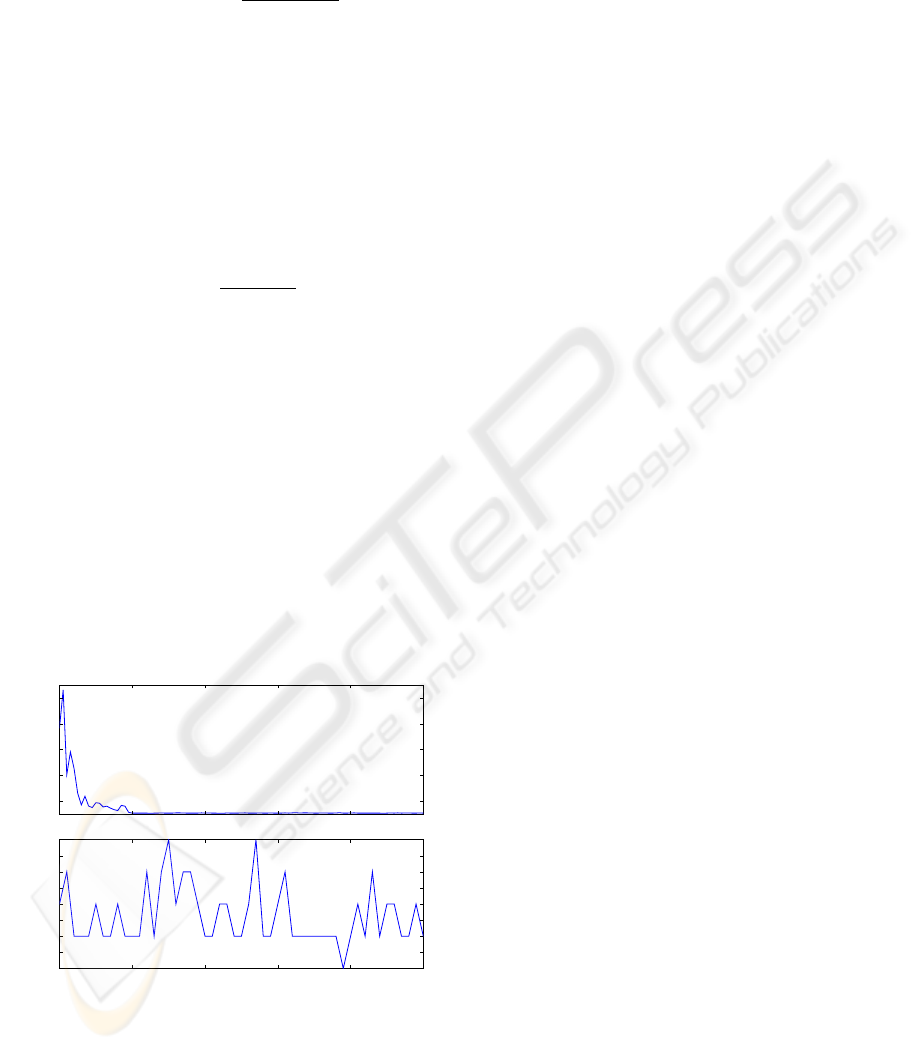
Figure 3, shows the result of the simulation, show-
ing the fact that the number of steps for reaching the
goal decrease up to a constant number of steps mean-
ing that this is the near optimal strategy for controlling
the agent.
0 20 40 60 80 100
episode num
200
400
600
800
1000
steps to reach the goal
50 60 70 80 90 100
last 50 episodes
105.0
105.5
106.0
106.5
107.0
107.5
108.0
108.5
109.0
steps to reach the goal
Figure 3: Mountain Car experimental results.
In Figure 3(Top) it can be seen that the number of
steps to reach the goal in the firsts episodes is near
1000 and in the subsequent episodes this step num-
ber decreases considerably, indeed, Figure 3(Bottom)
shows that the systems arrives to a stable configura-
tion around 107 steps per episode. An additional ob-
servation is that the speed of learning is high, from
the episode number 20, the system is practically sta-
bilized around the 107 steps per episode.
4 CONCLUSIONS AND FURTHER
WORK
A general framework for the problem of coordination
of multiple competing goals in dynamic environments
for physical agents has been presented. This approach
to goal coordination is a novel tool to incorporate a
deep coordination ability to pure reactive agents.
This framework was tested on two test problems
obtaining satisfactory results. Future experiments are
planed for a wide range of problems including differ-
ential games, humanoid robotics and modular robots.
Also we are interested in the study of methods for
reinforcement learning better suited for continuous
input states and multiple continuous actions. Usu-
ally a discretization of input and output variables is
produced but in other cases a better result could be
approximated if the problem were modeled by means
continuous states, generating more robust systems.
REFERENCES
Albus, J. (1975). A new approach to manipulator control:
The cerebellar model articulation controller (cmac). J.
of Dynamic Sys., Meas. and Control, pages 220–227.
Fonseca, C. M. and Fleming, P. J. (1995). An overview
of evolutionary algorithms in multiobjective optimiza-
tion. Evolutionary Computation, 3(1):1–16.
Isaacs, R. (1999). Differential Games. Dover Publications.
Passino, K. (2005). Biomimicry for Optimization, Control,
and Automation. Springer Verlag.
Sutton, R. (2006). Reinforcement learning and artificial in-
telligence. http://rlai.cs.ualberta.ca/RLAI/rlai.html.
Sutton, R. and Barto, A. (1998). Reinforcement Learning,
An Introduction. MIT Press.
Sutton, R. S. (1996). Generalization in reinforcement learn-
ing: Successful examples using sparse coarse coding.
In Touretzky, D. S., editor, Adv. in Neural Inf. Proc.
Systems, volume 8, pages 1038–1044. MIT Press.
Zitzler, E., Laumanns, M., Thiele, L., and Fonseca, C.
(2002). Why quality assessment of multiobjective op-
timizers is difficult. In Proc. GECCO 2002, pages
666–674.
DYNAMIC GOAL COORDINATION IN PHYSICAL AGENTS
159
