
MONTE CARLO LOCALIZATION IN HIGHLY SYMMETRIC
ENVIRONMENTS
Stephan Sehestedt, Frank E. Schneider
Research Establishment for Applied Sciences (FGAN)
Neuenahrer Strasse, 53343 Wachtberg, Germany
Keywords:
Monte Carlo Localization, MCL, Symmetric Environments, Two-Stage Sampling.
Abstract:
The localization problem is a central issue in mobile robotics. Monte Carlo Localization (MCL) is a popular
method to solve the localization problem for mobile robots. However, usual MCL has some shortcomings in
terms of computational complexity, robustness and the handling of highly symmetric environments. These
three issues are adressed in this work. We present three Monte Carlo localization algorithms as a solution to
these problems. The focus lies on two of these, which are especially suitable for highly symmetric environ-
ments, for which we introduce two-stage sampling as the resampling scheme.
1 INTRODUCTION
Localization is a crucial ability for a mobile robot in
order to be able to navigate. It is a key competence in
many successful robotic systems (see e.g. (S. Thrun,
2001), (S. Lenser, 2000)). Obviously, having a good
idea of ones position is also a prerequisite for decision
making and interaction with the environment. The
localization problem is often divided into three sub-
problems. The most basic problem is position track-
ing, where the robot starts with a known initial posi-
tion and just has to keep track of its pose. Whereas
global localization requires the robot to localize itself
from scratch. The most complex subproblem is the
kidnapped robot problem. Here the mobile unit has
to estimate its pose with a wrong initial believe. All
three subproblems can be solved with a particle fil-
ter algorithm (L. Ronghua, 2004), (Fox, 2003) and
(S. Lenser, 2000).
Here we also consider a fourth subproblem: Highly
symmetric environments. The basic particle filter of-
ten fails to localize a robot when there are a lot of
symmetries in the environment (L. Ronghua, 2004).
Therefore, it is necessary to introduce a technique that
allows to track multiple distinct positions on the map.
Symmetric environments need to be considered for
many mobile robot applications. Examples are robots
for surveillance in office buildings, where we fre-
quently find symmetries. We observe the same sit-
uation for different kinds of buildings. Furthermore,
robots operating in sewers and other tunnel like envi-
ronments may have to deal with ambiguities.
In the past years several approaches to Monte Carlo
localization had been proposed. Most of these fail
in symmetric environments (Fox, 2003), (S. Lenser,
2000) and (S. Thrun, 2001) or use large sample sets
(A. Milstein, 2002). A lot of research deals with the
efficient use of the samples, e.g. (S. Lenser, 2000), in
order to use small sample sets and only a few publi-
cations are concerned with variable sample set sizes
(L. Ronghua, 2004) and (Fox, 2003).
In this work we present three algorithms to solve
the localization problem based on Monte Carlo Meth-
ods. The first is derived from Dieter Fox’s KLD-
Sampling (Fox, 2003) and includes a procedure simi-
lar to Sensor Resetting Localization (S. Lenser, 2000).
We call this method KLD-Sampling with Sensor Re-
setting (KLD-SRL). The other two algorithms use
two-stage sampling for resampling in order to master
highly symmetric environments.
The remainder of this paper is organized as fol-
lows. Section 2 summarizes Monte Carlo Localiza-
tion. Section 3 outlines related work. Section 4 intro-
duces an efficient and robust localization algorithm
based on KLD-Sampling. Furthermore, in Section 5
we present an extension to MCL to handle symmet-
ric environments and show how to include it into the
schemes of existing MCL algorithms. Finally, In sec-
tion 7 we show the experimental results followed by
the conclusions.
2 MONTE CARLO
LOCALIZATION
Monte Carlo Localization (MCL) is a Bayesian ap-
proach to localization. There are numerous publica-
249
Sehestedt S. and E. Schneider F. (2006).
MONTE CARLO LOCALIZATION IN HIGHLY SYMMETRIC ENVIRONMENTS.
In Proceedings of the Third International Conference on Informatics in Control, Automation and Robotics, pages 249-254
DOI: 10.5220/0001215802490254
Copyright
c
SciTePress

Table 1: The three steps of the MCL algorithm.
1. Prediction: Draw x
i
t
∼ p(x
i
t
| x
i
t−1
, u
t−1
).
2. Update: Compute the importance factors ω
i
t
=
ηp(y
t
| x
i
t
), with η being a normalization factor
to ensure that the weights sum up to 1. Here, y
t
is a sensor reading at time t.
3. Resample.
tions presenting Monte Carlo Methods in detail, ex-
amples are (A. Doucet, 2000) and (S. Arulampalam,
2002). The belief is represented by a set of weighted
samples X(t) = hx
i
t
, ω
i
t
| i = 1, ..., Ni, where each
x
i
t
is a possible position of the robot and ω
i
t
the ac-
cording importance factor at time step t. The calcula-
tion of the posterior probability distribution consists
of three steps. Prediction, update and resampling.
Prediction is done by moving the samples in the
prior distribution as specified by the motion model.
Then the weights are calculated, using a sensor
model. Finally, in the additional resampling step, par-
ticles with low weight are replaced by those with sig-
nificant weight. Doing this, the samples get concen-
trated in areas of high probability. The downside is,
that this procedure can lead to premature convergence
in ambiguous situations (A. Bienvenue, 2002). For
more details on resampling see (A. Doucet, 2000).
MCL is summarized in table 1.
2.1 Discussion of MCL
Beside the very appealing attributes of particle filters
(S. Arulampalam, 2002), there are some issues that
need to be taken into account. Firstly, the basic parti-
cle filter uses large numbers of particles, what results
in high computational effort. Above this, MCL is
not able to track multiple hypotheses stable, but con-
verges to exactly one position. This can be harmful,
as we loose track of possibly right positions and do
not take these into account for pathplanning. Finally,
the basic particle filter recovers from localization fail-
ure very slowly.
3 RELATED WORK
3.1 Sensor Resetting Localization
Sensor Resetting Localization (SRL) is an extension
to Monte Carlo Localization (S. Lenser, 2000). In
each time step, a number of particles is replaced with
samples drawn from the sensor model. Using the
equation
Ns = (1 −
˜
P
P
t
) ∗ N (1)
we determine how many samples are to be replaced.
With
˜
P =
P
N
i=0
ω
i
t
/N and P
t
the probability thresh-
old, that can be adjusted to let the algorithm react
more or less sensitive. The logic behind this pro-
cedure is, that if the particles have a high average
weight, we can be certain that most samples are in
regions of high probability. If the average weight is
low, we can conclude that many particles are in un-
likely positions. Then we try to replace a number of
samples by sampling from the sensor model.
Therefore, we draw the new samples according to
the most recent sensor reading. Hence, these particles
are in areas of high probability. The problem with this
procedure is, that it may be very difficult to sample
from p(y
i
t
| x
i
t
) (S. Thrun, 2001).
SRL is mathematically questionable as it simply re-
moves a number of particles and replaces them with
new samples, as already mentioned in (S. Thrun,
2001).
4 ADAPTIVE PARTICLE FILTERS
4.1 KLD-Sampling
Variable sample set sizes allow us to adjust the num-
ber of particles to the complexity of the problem.
Clearly, we need much more particles for global lo-
calization than for tracking (Fox, 2003). Following
this logic, KLD-Sampling adjusts the number of par-
ticles based on the quality of the approximation of the
posterior distribution. We now give a brief description
of KLD-Sampling as introduced by Dieter Fox (Fox,
2003).
It is assumed that the true posterior is given by a
discrete, piecewise constant distribution. Then it can
be guaranteed that with probability 1 − δ the distance
between the true posterior and the sample-based ap-
proximation is less than ǫ.
For this, an approximation of the Kullback-Leibler
distance is used. We compute the number N of sam-
ples that is needed for the approximation based on the
number k of bins with support (Fox, 2003).
N =
k − 1
2ǫ
1 −
2
9(k − 1)
+
q
2
9(k−1)
z
1−δ
3
(2)
z
1−δ
is the upper 1−δ quantile of the standard normal
distribution. Then N relies on the inverse of the error
bound ǫ and is in the first order linear to k. To estimate
the number k of bins with support we used a fixed
ICINCO 2006 - ROBOTICS AND AUTOMATION
250

Table 2: The KLD-SRL algorithm.
1. Prediction: Draw x
i
t
∼ p(x
i
t
| x
i
t−1
, u
t−1
).
2. calculate N according to (2).
If N > N old:
draw N − Nold samples from p(y
i
t
| x
i
t
).
3. Update: Compute the importance factors ω
i
t
=
p(y
t
| x
i
t
).
4. normalize weights to sum up to 1.
5. Resample.
spatial grid, where a grid cell has support if at least
one particle lies in that cell.
It is easy to integrate KLD-Sampling into the parti-
cle filter scheme. In the prediction phase we count the
number of bins with support. If a sample falls into an
empty bin, we increase k. With each processed sam-
ple N is updated according to equation 2. Sampling
is stopped as soon as the number of samples reaches
N. For a complete description of this method refer to
(Fox, 2003).
4.2 KLD-Sampling with Sensor
Resetting
KLD-Sampling still leaves one bottleneck. While
global localization and when localization errors oc-
cur we have to use large numbers of particles. This
comes from the fact that new samples are uniformly
distributed over the state space. This is very ineffi-
cient in applications where it is possible to sample
from the sensor model p(y
t
| x
i
t
).
For this, we remember the number of samples we
used in the last step. We then compute N according to
equation (2) after the prediction phase. If N is larger
than the number of samples we used in the last time
step we add new samples to the sample set. The newly
generated samples are not just uniformly distributed
over the map but they are generated according to the
most recent sensor reading.
Sampling from the sensor model can be a very dif-
ficult task depending on the sensors one wants to use.
In this work we focused on laser range finders. For a
defined number of positions on the map, we syntheti-
cally produce the joint probability distribution p(y, x)
that contains the information about the occurrence of
a sensor reading y on a certain position x on the map.
This distribution is represented by a piecewise con-
stant distribution using a kd-tree.
In this way we place these particles in areas of high
probability and ignore areas of low probability. This
allows us to reduce the maximum size of the sample
set to a few hundred particles.
5 CLUSTERED PARTICLE
FILTERS
Usual MCL and KLD-Sampling often fail to correctly
localize a robot in ambiguous situations. Both meth-
ods prematurely converge to possibly wrong positions
on the map. As soon as the robot leaves the symmet-
ric parts of the environment, KLD-Sampling quickly
recovers from the localization failure.
Nevertheless, the pathplanner had possibly wrong
data about the pose before recovery. This may have
fatal consequences for the mobile unit. In the follow-
ing we describe the proposed algorithms for localiz-
ing a mobile robot in symmetric environments.
5.1 Background
In this section we present the mathematical back-
ground of our approach to Monte Carlo Localization
with clustering.
Using Sequential Importance Sampling (SIS), we
take account of the mismatch between the proposal
distribution and the target distribution (S. Thrun,
2001). In usual SIS the update equation for the im-
portance factors can be shown to be (S. Arulampalam,
2002)
ω
i
t
=
p(y
t
| x
i
t
)p(x
i
t
| x
i
t−1
)p(x
i
0:t−1
| y
0:t−1
)
q(x
i
t
| x
i
0:t−1
, y
1:t
)q(x
i
0:t−1
| y
1:t−1
)
(3)
with the numerator being the target distribution and
the denominator the proposal distribution. Seeing that
q(x
i
t
| x
i
0:t−1
, y
1:t
) = q(x
i
t
| x
i
t−1
, y
t
) we can calcu-
late the weights according to
ω
i
t
= η
p(y
t
| x
i
t
)p(x
i
t
| x
i
t−1
)
q(x
i
t
| x
i
t−1
, y
t
)
(4)
η is a normalizing constant, which ensures that the
weights sum up to 1. In that way, ω
i
t
is only de-
pendent on x
i
t
, y
t
, and y
t−1
. For our clustering ap-
proach we have to take account of the existence of the
clusters. Using a modified proposal distribution, we
have a function η(x
i
t
) which calculates the normaliz-
ing factor for the sample x
i
t
depending on the asso-
ciated cluster in which x
i
t
lies, in order to consider
multiple hypotheses.
ω
i
t
= η(x
i
t
)
p(y
t
| x
i
t
)p(x
i
t
| x
i
t−1
)
q(x
i
t
| x
i
t−1
, y
t
)
(5)
Consequently, we use the following equation to
compute the weights of the samples.
MONTE CARLO LOCALIZATION IN HIGHLY SYMMETRIC ENVIRONMENTS
251

ω
i
t
= η(x
i
t
)p(y
t
| x
i
t
) (6)
For C
j
t
being the sum of weights of the jth cluster
η(x
i
t
) = 1/C
j
t
(7)
This method allows us to use a procedure simi-
lar to Two-Stage Cluster Sampling as our resampling
scheme. In Two-Stage Cluster Sampling one divides
the whole sample set into clusters. In the first stage, a
cluster is randomly drawn. Then, in the second stage,
the actual sample is drawn (J. Hartung, 1989). Here
we first draw a cluster and then apply systematic re-
sampling on the individual particles in that cluster.
Hence, we draw samples from all clusters and there-
fore are able to keep track of multiple hypotheses.
Note, that we actually draw each of the clusters. If we
only detect one cluster, the resampling procedure be-
haves exactly like usual (systematic) resampling. Fur-
thermore, the association of a sample with a cluster is
determined in every time step. Thus, a sample can
be associated with different clusters in different time
steps.
5.2 Clustering
In the following, we present an extension to Monte
Carlo localization that allows for adequate localiza-
tion in highly symmetric environments as frequently
occurring in office like environments. Furthermore, it
is shown how to incorporate this into the functionality
of Sensor Resetting Localization and KLD-Sampling
with Sensor Resetting.
In order to use two-stage sampling, we need to de-
termine clusters in the sample set. Clustering is a well
known technique to classify data and build groups of
similar objects (W. Lioa, 2004). Here we use cluster-
ing to find groups of particles that occupy the same
area in the state space. Doing this, we try to extract
significant clusters that represent a possible position
of our robot.
When choosing a clustering method, we mainly
need to care about two things. The speed of this
routine and the accuracy. Regarding the speed, grid-
based algorithms are a good choice (W. Lioa, 2004).
For us, a clustering algorithm is accurate, if it finds
all significant particle clusters. That are those clusters
with a high average weight. Clusters with low weight
are not likely to represent the correct pose and can
therefore be discarded. That implies, that the output
of the clustering procedure only includes the signifi-
cant clusters.
We used a fixed spatial grid for a first estimate
of the clusters. Here a coarse grid of approximately
2 m ∗ 2 m ∗ 45 degree is sufficient and since we have
to do the clustering for just a few hundred samples it
is fast as well. If we detect more than one cluster, it
is checked if clusters can be fused. This is the case,
if clusters are in close proximity of each other in the
state space.
Thereby, the importance factors are computed ac-
cording to equation (6). In that way, we do not loose
possible positions while resampling. A cluster is con-
sidered significant if it’s weight is above a manually
chosen threshold. This method showed to be stable
and accurate. Moreover, it allows us to simply dis-
tribute the free samples from clusters with low weight
over the significant clusters. While resampling these
samples are replaced with the high weighted particles
of the according cluster. Alternatively, one can re-
place these samples by newly generated ones.
5.3 Clustered Sensor Resetting
Localization
To incorporate two-stage sampling we need to regard
the fact that SRL simply replaces particles in the sam-
ple set if needed. Thus, we cannot guarantee that all
clusters will still exist after this replacement. In order
to exclude this case, we disable the replacement of
particles whenever we find more than one significant
cluster. The algorithm is summarized in table 3.
The intuition behind CSRL is as follows. When the
robot gets kidnapped while our filter is tracking mul-
tiple distinct hypotheses, we observe the following.
The weights of the clusters become negligible and are
therefore not considered significant any more. Thus,
we do regard all samples as though they were in one
cluster. We then can calculate a number of samples
to be replaced according to Sensor Resetting Local-
ization. The newly generated particles are distributed
according to the most recent sensor reading. Then, for
the new sample set, clustering is done and it is decided
if we have to track multiple or a single position.
In this way, we are able to combine the ability to
track multiple hypotheses stable with the advantage
of using small sample sets.
5.4 Clustered KLD-Sampling with
Sensor Resetting
Clustered Sensor Resetting Localization still suffers
from using a sample set of constant size. Thus, we
are not taking account of the different complexities of
the localization problem. To overcome this issue, we
developed a method to combine two-stage sampling
with KLD-SRL.
Analogous to KLD-SRL the number of particles is
adjusted according to equation (2). Only, if we detect
more than one significant cluster, we do not allow the
number of samples to be reduced. So we can guaran-
tee that we won’t loose any of the detected clusters.
As soon as there is only one cluster left, the number
ICINCO 2006 - ROBOTICS AND AUTOMATION
252
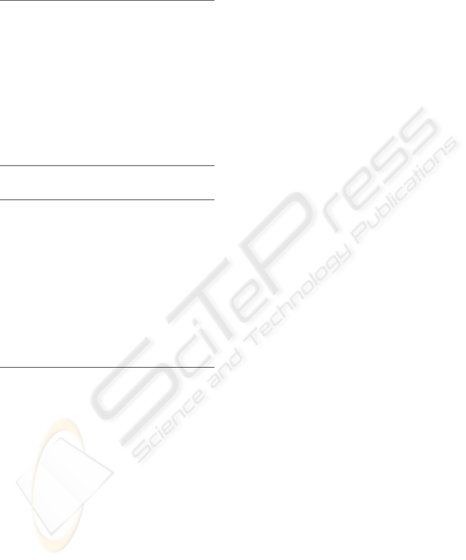
Table 3: The CSRL algorithm.
1. Prediction: Draw x
i
t
∼ p(x
i
t
| x
i
t−1
, u
t−1
).
2. Update: Compute the importance factors ω
i
t
=
p(y
t
| x
i
t
).
3. Normalize weights to sum up to 1.
4. Determine the number of significant clusters.
5. Resample using two-stage sampling.
6. If there is one cluster:
Compute Ns according to equation (1).
If Ns > 0: Replace Ns samples with sam-
ples drawn from p(y
i
t
| x
i
t
).
Table 4: The Clustered KLD-SRL algorithm.
1. Prediction: Draw x
i
t
∼ p(x
i
t
| x
i
t−1
, u
t−1
).
2. calculate N according to (2).
3. If N > Nold:
draw N − Nold samples from p(y
i
t
| x
i
t
).
4. If N < Nold and number of clusters is one:
Decrease number of samples to N.
5. Update: Compute the importance factors ω
i
t
=
p(y
t
| x
i
t
).
6. normalize weights to sum up to 1.
7. Resample using two-stage clustering.
of samples can be adjusted in the usual way. Note,
that the number samples can still be increased while
tracking multiple clusters and thus, allowing to find
more clusters.
In ambiguous situations we usually have a number
of significant clusters that we do not want to disappear
prematurely. As soon as we detect distinct features in
the environment, all but one cluster will have negli-
gible weights and therefore be merged into the one
cluster with high weight. Then, the number of sam-
ples can be decreased again.
Clustered KLD-SRL joins the advantages of using
a small and variable sample set and the ability to track
multiple positions over extended periods of time. Ex-
periments show this algorithm to be accurate and ro-
bust. The algorithm is summarized in table 4.
6 EXPERIMENTAL RESULTS
In this section we present the results of our exper-
iments. Due to the fact that it is very difficult to
obtain quantitative results in real world experiments,
we focus on simulations. Different maps have been
used to test accuracy and tracking multiple hypothe-
ses. Simulations were conducted on a 1.7 GHz Pen-
tium 4 computer with 512 MB of memory.
Firstly, we ran simulations with KLD-SRL. Since
this algorithm is not able to cope with symmetric en-
vironments properly, accuracy, robustness and speed
are the measures of interest. In situations like the one
illustrated in figures 1(a) and 1(b) KLD-SRL usually
fails. The average localization failure was approxi-
mately 3 cm, with a mean update time of 0.03 sec-
onds. Kidnapping experiments revealed the time for
recovery from localization failure to be approximately
2 seconds in the average. Further experiments showed
that the according values are in the same magnitude
for CSRL and Clustered KLD-SRL.
To test the ability of tracking multiple hypotheses
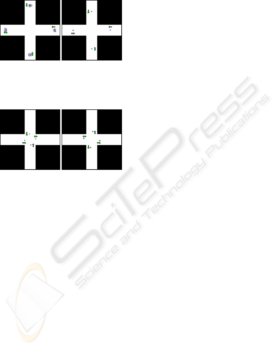
stable over extended periods of time, we generated
a completely symmetric map consisting of a cross
shaped area of approximately 15 m ∗ 15 m (figures 1
and 2). The green arrows indicate the estimated head-
ing of the robot according the position estimate. This
looks the same for Clustered Sensor Resetting Lo-
calization and Clustered KLD-Sampling with Sensor
Resetting. Methods that do not facilitate techniques
to handle symmetries converge to one single position
and therefore this estimate is wrong in most cases.
Figure 1(a) shows the initialization of the filter,
where all particles are distributed according to the
most recent sensor reading. Thus, the samples cover
four possible positions on the map. Since there is no
way to figure out which of these poses is the right
one, the filter keeps track of all of them (figures 1(a)
to 2(b)). Even as the estimates cross in the middle, we
do not loose any of them.
Furthermore, we conducted experiments with maps
of office buildings, where we observe a lot of symme-
tries and asymmetries. Global localization was per-
formed at random starting points and was success-
fully done in all cases. Above this, we frequently kid-
napped the robot and let it relocalize itself. Most of
the time we placed it on symmetric parts of the map
and kidnapping was also done while the filter tracked
multiple hypotheses.
In these experiments, relocalization was usually
performed within 2 seconds and as soon as the robot
left the symmetric part of the environment, the fil-
ter converged to the correct position. Thus, both,
CSRL and Clustered KLD-SRL, are able to localize a
robot in highly symmetric environments and thereby
showed to be very robust and accurate.
Regarding computational complexity, CSRL is in-
MONTE CARLO LOCALIZATION IN HIGHLY SYMMETRIC ENVIRONMENTS
253
(a) (b)
Figure 1: CSRL: a) After initialization on a cross shaped
symmetric map. The green arrows denote the actual head-
ing of the robot, according to the four possible positions. b)
The robot moves. Simulated data.
(a) (b)
Figure 2: CSRL: a) The four distinct position estimates
come to close proximity in the middle of the cross. b) The
robot moves on. Simulated data.
ferior, since it uses a sample set of constant size.
The drawback of using variable sample set sizes is,
that sometimes we need significantly more computa-
tion time. Thus, we always have to regard the worst
case or design the robotic system in a way, that some
processes can sleep for a while without affecting the
usual operation too much.
7 CONCLUSIONS
The focus of this work is on handling highly symmet-
ric environments with a particle filter algorithm. Nev-
ertheless, computational complexity and robustness
are still important issues, that need to be regarded.
We introduced a resampling scheme that is easy to
integrate into a particle filter.
Furthermore, we presented two algorithms that are
able to localize a mobile unit correctly in symmetric
environments at all times. CSRL uses small but con-
stant sample sets. Therefore, CKLD-SRL is superior
to this method, for its use of variable sample sets. Ex-
perimental results show the good quality of the posi-
tion estimate and high robustness produced by these
methods.
Further research is concerned with the viability of
such methods for 3D/6D localization. Furthermore,
we are interested in using such filters for multi target
tracking (A. Kraeussling, 2005).
REFERENCES
A. Bienvenue, M. Joannides, J. B. E. F. O. F. (2002). Nich-
ing in monte carlo filtering algorithms. In Selected
Papers from the 5th European Conference on Artifi-
cial Evolution, pages 19–30, London, UK. Springer-
Verlag.
A. Doucet, S.J. Godsill, C. A. (2000). On sequen-
tial simulation-based methods for bayesian filtering.
Statistics and Computing, 10:197–208.
A. Kraeussling, F. E. Schneider, D. W. (2005). Track-
ing extended moving objects with a mobile robot. In
Proceedings of the IEEE International Conference on
Robotics and Automation, volume 2, pages 126 – 133.
A. Milstein, J. N. S
´
anchez, E. T. W. (2002). Robust global
localization using clustered particle filtering. In Eigh-
teenth national conference on Artificial intelligence,
pages 581–586. American Association for Artificial
Intelligence.
Fox, D. (2003). Adapting the sample size in particle fil-
ters through kld-sampling. International Journal of
Robotics Research (IJRR), 22:985–1003.
J. Hartung, B. Elpelt, K. K. (1989). Statistik - Lehr- und
Handbuch der angewandten Statistik. Oldenburg.
L. Ronghua, H. B. (2004). Coevolution based adaptive
monte carlo localization (ceamcl). International Jour-
nal of Advanced Robotic Systems, 1(3):183–190.
S. Arulampalam, S. Makell, N. G. T. C. (2002). A tutorial
on particle filters for online non-linear/non-gaussian
bayesian tracking. IEEE Transactions on Signal Pro-
cessing, 50:174–188.
S. Lenser, M. V. (2000). Sensor resetting localization for
poorly modelled mobile robots. In Proceedings of the
IEEE International Conference on Robotics and Au-
tomation.
S. Thrun, D. Fox, W. B. F. D. (2001). Robust monte carlo
localization for mobile robots. Artificial Intelligence,
128(1-2):99–141.
W. Lioa, Y. Liu, A. C. (2004). A grid-based clustering algo-
rithm using adaptive mesh refinement. In Proceedings
of the 7th Workshop on Mining Scientific and Engi-
neering Datasets, pages 288 – 292.
ICINCO 2006 - ROBOTICS AND AUTOMATION
254
