
REDUCING ACCUMULATED ERRORS IN EGO-MOTION
ESTIMATION USING LOCAL BUNDLE ADJUSTMENT
Akihiro Sugimoto
National Institute of Informatics
Chiyoda, Tokyo 101-8430, Japan
Tomohiko Ikeda
Chiba University
Inage, Chiba 263-8522, Japan
Keywords:
Accumulated errors, ego-motion estimation, bundle adjustment, fixation control, computer vision.
Abstract:
Incremental motion estimation methods involve a problem that estimation accuracy gradually becomes worse
as the motion trajectory becomes longer and longer. This is due to accumulation of estimation errors incurred
in each estimation step. To keep estimation accuracy stable even for a long trajectory, we propose to locally
apply the bundle adjustment to each estimated motion so that the modified estimation becomes geometrically
consistent with time-series frames acquired so far. To demonstrate the effectiveness of this approach, we em-
ploy an ego-motion estimation method using the binocular fixation control, and show that (i) our modification
of estimation is statistically significant; (ii) in order to reduce estimation errors most effectively, three frames
are optimal for applying the bundle adjustment; (iii) the proposed method is effective in the real situation,
demonstrating drastic improvement of accuracy in estimation for a long motion trajectory.
1 INTRODUCTION
In the wearable computer environment (Clarkson et
al., 2000) understanding where a person was and
where the person is/was going is a key issue (Aoki
et al., 2000; Davison et al., 2003) for just-in-time
teaching, namely, for providing useful information
at teachable moment. In the robot vision, on the
other hand, the SLAM (Simultaneous Localization
and Mapping) problem(Dissanayake et al., 2001;
Guivant and Nebot, 2001; Thrun, 2002), in particular,
mobile robot navigation and docking require the ro-
bot localization, the process of determining and track-
ing the position (location) of mobile robots relative to
their environments (Davison and Murray, 1998; DeS-
ouza and Kak, 2002; Nakagawa et al., 2004; Sumi et
al., 2004; Werman et al., 1999). Computing three-
dimensional camera motion from image measure-
ments is, therefore, one of the fundamental problems
in computer vision and robot vision.
Most successful vision-based approaches to esti-
mating the position and motion of a moving robot
usually employ the stereo vision framework. For ex-
ample, Davison-Murray(Davison and Murray, 1998)
assumed planar motions and proposed a method that
reconstructs 3D points as landmarks and that im-
poses on the points geometrical constraints derived
from planar motions. Gonc¸alves–Ara
´
ujo(Gonc¸alves
and Ara
´
ujo, 2002) proposed a method for estimat-
ing motions that uses information obtained from op-
tical flows and a 3D point reconstructed by stereo vi-
sion. Molton–Brady (Molton and Brady, 2003), on
the other hand, proposed a method that reconstructs
3D points and uses their correspondences before and
after a motion for the motion estimation.
When we employ the stereo vision framework,
however, we have to make two cameras share the
common field of view and, moreover, establish fea-
ture correspondences across the images captured by
two cameras. This kind of processing has difficulty
in its stability. In addition, keeping the baseline dis-
tance wide is hard when we mount cameras on a ro-
bot or wear cameras. Therefore, accuracy of motion
estimation is limited if we employ the stereo vision
framework.
To overcome such problems, Sugimoto et
al.(Sugimoto et al., 2004; Sugimoto and Ikeda,
2004) introduced the binocular independent fixation
control(Sugimoto et al., 2004) (Fig. 1) to two active
cameras, and proposed a method for incrementally
estimating camera motion that ensures estimation
accuracy independent of the baseline distance of
the two cameras. In the method, the correspon-
dence of the fixation point over last two frames
418
Sugimoto A. and Ikeda T. (2006).
REDUCING ACCUMULATED ERRORS IN EGO-MOTION ESTIMATION USING LOCAL BUNDLE ADJUSTMENT.
In Proceedings of the Third International Conference on Informatics in Control, Automation and Robotics, pages 418-425
DOI: 10.5220/0001213904180425
Copyright
c
SciTePress

obtained through the camera control together with
line correspondences(Sugimoto et al., 2004) or
optical flows(Sugimoto and Ikeda, 2004) plays a key
role in motion estimation. This method, however,
has a problem that estimation accuracy gradually
becomes worse as the motion trajectory becomes
longer and longer. This is because estimation errors
incurred in each estimation step are accumulated and
accumulated errors cannot be ignored in the case of a
long trajectory. This problem is commonly involved
in incremental estimation of parameters.
In the area of camera calibration, in particular cal-
ibration of multiple cameras, on the other hand, pa-
rameter estimation is usually formulated as a nonlin-
ear least squares problem whose cost function is de-
fined in terms of reprojection errors. Two steps are
then iterated until convergence is observed: searching
for parameters minimizing the cost function and re-
constructing 3D feature coordinates using estimated
parameters to compute reprojection errors for a cost
function. This approach appears long ago in the pho-
togrammetry and geodesy literatures and is referred to
the bundle adjustment (Hartley and Zisserman, 2000;
Triggs et al., 2000).
In this paper, we propose a method that incorpo-
rates the bundle adjustment to ego-motion estima-
tion method using the binocular independent fixa-
tion control in order to reduce estimation errors in
each step and, as a result, to reduce accumulated er-
rors in estimation. The bundle adjustment is origi-
nally applied to all estimated parameters after all es-
timation steps are finished to modify all the parame-
ters simultaneously. In this sense, the bundle adjust-
ment is a batch process and not suitable for an incre-
mental process like ego-motion estimation. To solve
this contradiction, we here employ an approach of
the bundle adjustment application to parameters es-
timated within local computation (Zhang and Shan,
2001; Zhang and Shan, 2003). We locally apply the
bundle adjustment to each estimated motion so that
the modified estimation becomes geometrically con-
sistent with time-series images captured so far. This
modification keeps the estimation method incremen-
tal and, at the same time, reduces estimation errors in-
curred in each estimation step and drastically reduces
accumulated errors. The contributions of this paper
to ego-motion estimation are summarized in three im-
portant respects: (i) we show that our modification of
estimation is statistically significant; (ii) we show that
in order to reduce estimation errors most effectively,
three frames are optimal for applying the bundle ad-
justment; (iii) we demonstrate the effectiveness of the
proposed method in the real situation, showing dras-
tic improvement of accuracy in estimation for a long
motion trajectory.
Figure 1: Binocular independent fixation control.
2 BINOCULAR INDEPENDENT
FIXATION CONTROL
We here review the ego-motion estimation method
that uses the binocular fixation control(Sugimoto and
Ikeda, 2004). We note that in the binocular fixation
control, each camera independently and automatically
fixates its optical axis to its own fixation point in 3D
and two fixation points are not necessarily the same.
Between a right camera and a left camera, we set
the right camera is the base. Moreover, for simplicity,
we assume that the orientation of the camera coordi-
nate system does not change even though we change
pan and tilt of the camera for the fixation control. This
means that only the ego motion causes changes in ori-
entation and translation of the camera coordinate sys-
tems. We also assume that the ego motion is identical
with the motion of the right-camera coordinate sys-
tem. We let the translation vector and the rotation ma-
trix to make the left-camera coordinate system iden-
tical with the right-camera coordinate system be T
in
and R
in
respectively. We also assume that the rotation
and the translation of the right-camera coordinate sys-
tem incurred by the ego motion are expressed as ro-
tation matrix R in the right-camera coordinate system
at time t and translation vector T in the world coordi-
nate system. We remark that the extrinsic parameters
between the two cameras as well as the intrinsic pa-
rameters of each camera are assumed to be calibrated
in advance.
We denote by v
t
r
the unit vector from the projection
center of the right camera toward the fixation point of
the right camera in the right-camera coordinate sys-
tem at time t. The constraint on ego-motion parame-
ters follows from the fixation correspondence of the
right camera:
det
R
0
v
t
r
| R
0
Rv
t+1
r
| T
= 0,
where R
0
is the rotation matrix that makes the orien-
tation of the world coordinate system identical with
the orientation of the right-camera coordinate system
at time t. Similarly, we obtain the following con-
straint on the ego-motion parameters from the fixation
REDUCING ACCUMULATED ERRORS IN EGO-MOTION ESTIMATION USING LOCAL BUNDLE ADJUSTMENT
419

correspondence of the left camera.
det
R
0
R
⊤
in
v
t
ℓ
| R
0
RR
⊤
in
v
t+1
ℓ
|
T − R
0
(R − I)R
⊤
in
T
in
= 0.
Here v
t
ℓ
is defined in the same way as v
t
r
.
Let q
t
r
be the coordinates of a point in the right-
camera image at time t, and u
t
r
be the flow vector at
the point. We then have the constraint on the ego-
motion parameters:
det
h
R
0
R(M u
t
r
+
e
q
t
r
) | R
0
e
q
t
r
| T
i
= 0, (1)
where
M =
1 0 0
0 1 0
⊤
,
e
q
t
r
= ((q
t
r
)
⊤
, f
r
)
⊤
and f
r
is the focal length of the right camera. In the
similar way, optical flow obtained from the left cam-
era gives us the constraint on the ego motion.
det[R
0
RR
⊤
in
(Mu
t
ℓ
+
e
q
t
ℓ
) | R
0
R
⊤
in
e
q
t
ℓ
|
T − R
0
(R − I)R
⊤
in
T
in
] = 0,
where q
t
ℓ
is a point in the left-camera image at time t
and u
t
ℓ
is the flow vector at the point. Note that
e
q
t
ℓ
is
defined by
e
q
t
ℓ
:=
(q
t
ℓ
)
⊤
f
ℓ
⊤
using the focal length
f
ℓ
of the left camera.
Ego motion has 6 degrees of freedom: 3 for a ro-
tation and 3 for a translation. The number of al-
gebraically independent constraints on the ego mo-
tion derived from two fixation correspondences, on
the other hand, is two. One algebraically indepen-
dent constraint is derived from each optical flow vec-
tor. We can therefore estimate ego motion if we have
optical-flow vectors at more than four points. Namely,
we form a simultaneous system of all the nonlinear
constraints above and then apply a nonlinear opti-
mization algorithm to solve the system. Parameters
optimizing the system give the estimation of ego mo-
tion.
3 LOCAL BUNDLE
ADJUSTMENT
The method reviewed in the previous section incre-
mentally estimates ego motion using last two frames
in each step. We cannot, however, guarantee that
the method estimates correct motion parameters due
to nonlinear optimization involved in estimation in
each step: we may be trapped by a locally optimal
solution. Even though the globally optimal solution
is obtained, we still have errors incurred by numeri-
cal computation and/or observation of fixation point
or optical flows. This means that we cannot ignore
the accumulation of errors incurred in each estimation
step and that estimation accuracy gradually becomes
worse as the motion trajectory becomes longer and
longer. As a result, geometrical inconsistency arises
in the relationship between the fixation point in the
current image and that in the other images captured
so far. We here modify estimated parameters using
the bundle adjustment so that such geometrical incon-
sistency does not occurs.
We assume that images are captured in discrete
time-series and that from time s to time t (t ≥ s + 2),
motion parameters between two frames are already
estimated. We denote by R
i,i+1
, T
i,i+1
the motion
parameters between time i and time i + 1 (i =
s, . . . , t − 1). Here, R
i,i+1
and T
i,i+1
are the rota-
tion matrix and the translation vector representing the
ego-motion from time i to time i + 1. We remark that
the fixation control enables us to obtain the correspon-
dences of fixation point images p
i
(i = s, . . . , t) from
time s to time t.
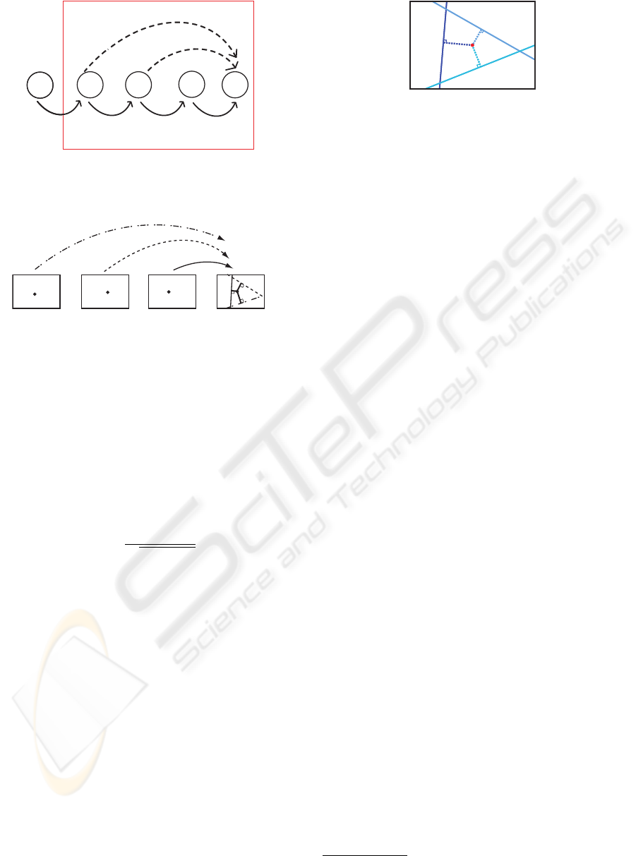
For an image at time t, we focus on last n images
including the image at time t (3 ≤ n ≤ t − s + 1).
We then apply the bundle adjustment to the n images.
Since motion parameters relating two frames are al-
ready estimated at each time, we can combine them to
obtain motion parameters R
j,t
and t
j,t
that relate the
images at time j and time t (t − n + 1 ≤ j ≤ t − 1)
(see Fig.2):
R
j,t
=
t−1
Y
i=j
R
i,i+1
, T
j,t
=
t−1
X
i=j
T
i,i+1
.
These parameters allow us to obtain in the image at
time t, the epipolar line corresponding to p
j
. From
the theoretical point of view, this epipolar line passes
through p
t
, however, estimation errors and/or their
accumulation cause the problem that the line does not
pass through the point p
t
as shown in Fig. 3. This in-
dicates that epipolar constraints are broken. In other
words, geometrical inconsistency arises in the rela-
tionship between the fixation point in the current im-
age and that in the time-series images captured so far.
In the image at time t, the epipolar line determined
by p
j
and R
j,t
, T
j,t
is expressed by
˜
x
⊤
E
j,t
˜
p
j
= 0, (2)
where
˜
x is the homogeneous coordinates of a point in
the image at time t,
˜
p
j
is the homogeneous coordi-
nates of p
j
and
1
E
j,t
:= [T
j,t
]
×
R
j,t
.
1
[T
j,t
]
×
is the 3 × 3 skew-symmetric matrix deter-
mined by T
j,t
. Namely, for any 3-dimensional vector y,
[T
j,t
]
×
y = T
j,t
× y is satisfied.
ICINCO 2006 - ROBOTICS AND AUTOMATION
420
t-4 t-2t-3 t-1 t
R
t-4,t-3
T
t-4,t-3
R
t-3,t-2
T
t-3,t-2
R
t-2,t-1
T
t-2,t-1
R
t-1,t
T
t-1,t
R
t-3,t
,T
t-3,t
R
t-2,t
,T
t-2,t
t-4 t-2t-3 t-1 t
R
t-4,t-3
T
t-4,t-3
R
t-3,t-2
T
t-3,t-2
R
t-2,t-1
T
t-2,t-1
R
t-1,t
T
t-1,t
R
t-3,t
,T
t-3,t
R
t-2,t
,T
t-2,t
Figure 2: Relationship between motion parameters to which
the local bundle adjustment is applied (the case of four
frames).
R
t-3,t
tt-1t-2t-3
T
t-3,t
R
t-2,t
T
t-2,t
R
t-1,t
T
t-1,t
Figure 3: Epipolar lines obtained by the current fixation
point and estimated parameters.
We can therefore evaluate errors of R
j,t
and T
j,t
us-
ing the displacement of
˜
p
t
from (2). We sum up dis-
placements of
˜
p
t
from each of the epipolar lines ob-
tained from the last (n − 1) images and then mod-
ify R
t−1,t
and T
t−1,t
so that modified parameters
minimize the summation of the displacements over
the concerned epipolar lines. Geometrical distance is
used to evaluate the displacement of a point from a
line (see Fig.4). The cost function to be minimized is
thus
t−1
X
j=t−n+1
˜
p
⊤
t
E
j,t
˜
p
j
q
a
2
j,t
+ b
2
j,t
2
, (3)
where (a
j,t
, b
j,t
, c
j,t
)
⊤
= E
j,t
˜
p
j
.
Modification of parameters R
t−1,t
, T
t−1,t
so that
modified parameters minimize (3) guarantees that the
epipolar constraints derived from the fixation point
and the last n frames are more strictly satisfied than
before. We remark that our modification is applied
only to R
t−1,t
, T
t−1,t
; the number of parameters to
be modified is independent of n. Accordingly, the
computational cost required for the modification does
not change even if we change the number of last
frames to be applied for the bundle adjustment.
As described above, our modification of estimated
parameters, i.e., applying the bundle adjustment in
each step only to last several frames, keeps geometri-
cal consistency with last frames captured so far. With
this modification, errors involved in the parameters
before the modification are reduced. This modifica-
tion thus suppresses the amount of accumulated er-
rors even for incremental estimations and significant
improvement of accuracy in estimation for a long tra-
p
t
p
t
Figure 4: Distance between the fixation point and its corre-
sponding epipolar lines.
jectory is expected. We finally remark that we mini-
mize the cost function using a nonlinear optimization
algorithm because (3) is nonlinear with respect to R
j,t
and T
j,t
.
4 EXPERIMENTS
We conducted experiments to estimate ego-motion
using the proposed method. We first quantitatively
evaluate improvement in reducing estimation errors
using simulated data. We also evaluate the number of
frames to which our local bundle adjustment should
be applied to reduce errors most effectively. We fi-
nally examine the proposed method using real images.
4.1 Numerical Evaluation Using
Simulated Data
We here test the proposed method using simulated
data. To see the effectiveness of the proposed method,
we implemented the method proposed by Sugimoto–
Ikeda(Sugimoto and Ikeda, 2004), called the compar-
ison method hereafter, and then evaluated how much
estimation errors are reduced by comparing the two
methods.
We first test the case of n = 3 in the previous sec-
tion, i.e., the case where the bundle adjustment is lo-
cally applied to last three frames and compare errors
estimated by the two methods.
The parameters used in the simulation are as fol-
lows. Two cameras are set with the baseline distance
of 1.0 where each camera is with 21
o
angle of view
and with the focal length
2
of 0.025. The two cameras
are in the same pose: the orientation of the camera
coordinate systems is the same. The size of images
captured by the cameras is 512 × 512 pixels.
We set a distance between two fixation points to be
10.0 and generated two fixation points in 3D for the
two cameras satisfying the distance. We note that the
depth of each fixation point was set 10.0 forward from
the projection center. We also randomly generated 3
points in 3D nearby each fixation point for the optical-
flow computation. The images of the two points were
2
When the baseline distance is 20cm, then the focal
length is 0.5cm, for example.
REDUCING ACCUMULATED ERRORS IN EGO-MOTION ESTIMATION USING LOCAL BUNDLE ADJUSTMENT
421
0
0.1
0.2
0.3
0.4
0.5
after
modification
before
modification
0
0.1
0.2
0.3
0.4
0.5
after
modification
before
modification
(a) translations (b) rotations
errors
Figure 5: Estimation errors in the case where the distance
between fixation points is 10 baseline.
within the window of 20 × 20 pixels whose center is
the image of the fixation point.
To obtain three time-series images, we generated
two steps of motion. For the first step, we randomly
generated a translation vector with the length of 0.25
and a rotation matrix where the rotation axis is verti-
cal and the rotation angle is within 1.0 degree. For the
second step, on the other hand, we rotated the trans-
lation vector generated in the first step around the Z
axis of the camera coordinate system where the ro-
tation angle was randomly selected between −1.0
o
and 1.0
o
. As for the rotation of the second step, we
just added rotation angle randomly selected between
−1.0
o
and 1.0
o
to the rotation angle of the first step.
Before and after the motion, we projected all the
points generated in 3D onto the image plane to ob-
tain image points that were observed in terms of pix-
els. To all the image points, we added Gaussian noise.
Namely, we perturbed the pixel-based coordinates in
the image by independently adding Gaussian noise
with the mean of 0.0 pixels and the standard devia-
tion of 2.0 pixels. Next, we computed optical flow of
the points generated nearby the fixation points to ob-
tain the flow vectors. We then applied our algorithm
to obtain ego-motion estimation: rotation matrix
b
R
and translation vector
b
T .
To evaluate errors in estimation, we computed ro-
tation axis
b
r (k
b
rk = 1) and rotation angle
b
θ from
b
R.
We then defined the evaluation of errors of
b
R and
b
T
by
||
ˆ
θ
ˆ
r − θr||
|θ|
,
||
ˆ
T − T ||
||T ||
,
where r (krk = 1) is the rotation axis and θ is the
rotation angle of the ground truth, and T is the true
translation vector (kT k = 0.25). We iterated the
above procedures 200 times and computed the aver-
age and the standard deviation of the errors over the
200 iterations.
The result is shown in Fig. 5. We see that esti-
mation errors are actually reduced by the proposed
method. From Fig. 5 (b), we observe little difference
in estimation errors between the proposed method
and the comparison method. As for the rotation es-
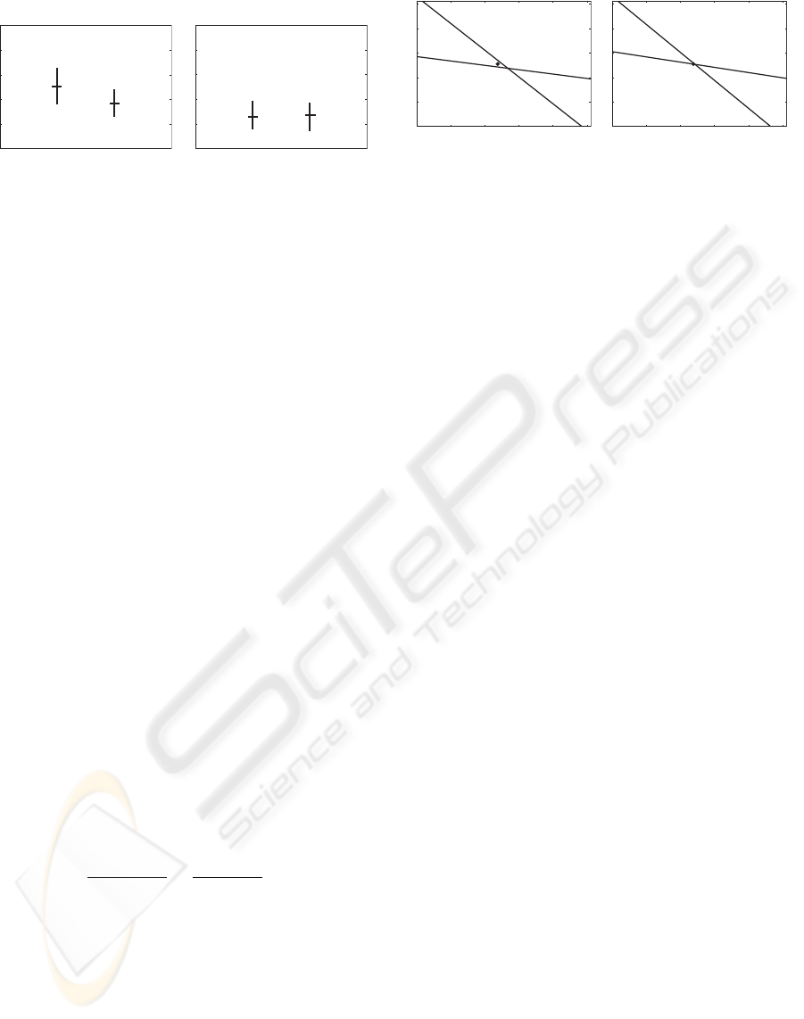
0
100
200
300
400
500
0 100 200 300 400 500
0
100
200
300
400
500
0 100 200 300 400 500
(a) before modification (b) after modification
Figure 6: Fixation point and its corresponding epipolar lines
before/after parameter modification.
timation, the comparison method is reported to real-
ize highly accurate estimation(Sugimoto and Ikeda,
2004). This is why little improvement is observed.
Fig.5 (a), on the other hand, shows the proposed
method actually reduces the average and also the stan-
dard deviation of estimation errors. To verify whether
or not this difference makes sense from the statisti-
cal point of view, we employed Welch’s test (Welch,
1938) with significance level of 5%. We then certified
that the difference is statistically significant.
We drew epipolar lines for a case among the 200
cases above, which are illustrated in Fig. 6. Fig.6
demonstrates that the distance between the epipolar
lines and the fixation point in the image becomes
smaller after the modification. In fact, we computed
the distances between the fixation point and the epipo-
lar lines and found that they are 10 pixels and 0.2 pix-
els before and after the modification, respectively. We
confirmed that in almost all the 200 cases, the dis-
tances between the fixation point and epipolar lines
are the same degree as this typical case.
We verified that values of the cost function actually
become smaller after the modification for all the 200
cases. A smaller value of the cost function, however,
does not always mean that more accurate estimation is
realized. This is because the case exists where a rota-
tion error and a translation error can cancel each other
in terms of the cost function. This implies that how-
ever close the cost function achieves zero, estimation
errors can exist and that we have a limitation of re-
ducing estimation errors. Considering these factors,
we may conclude that our modified estimation be-
comes geometrically consistent with last two frames
captured so far and that our proposed method signifi-
cantly improves accuracy in estimation, with keeping
the method incremental.
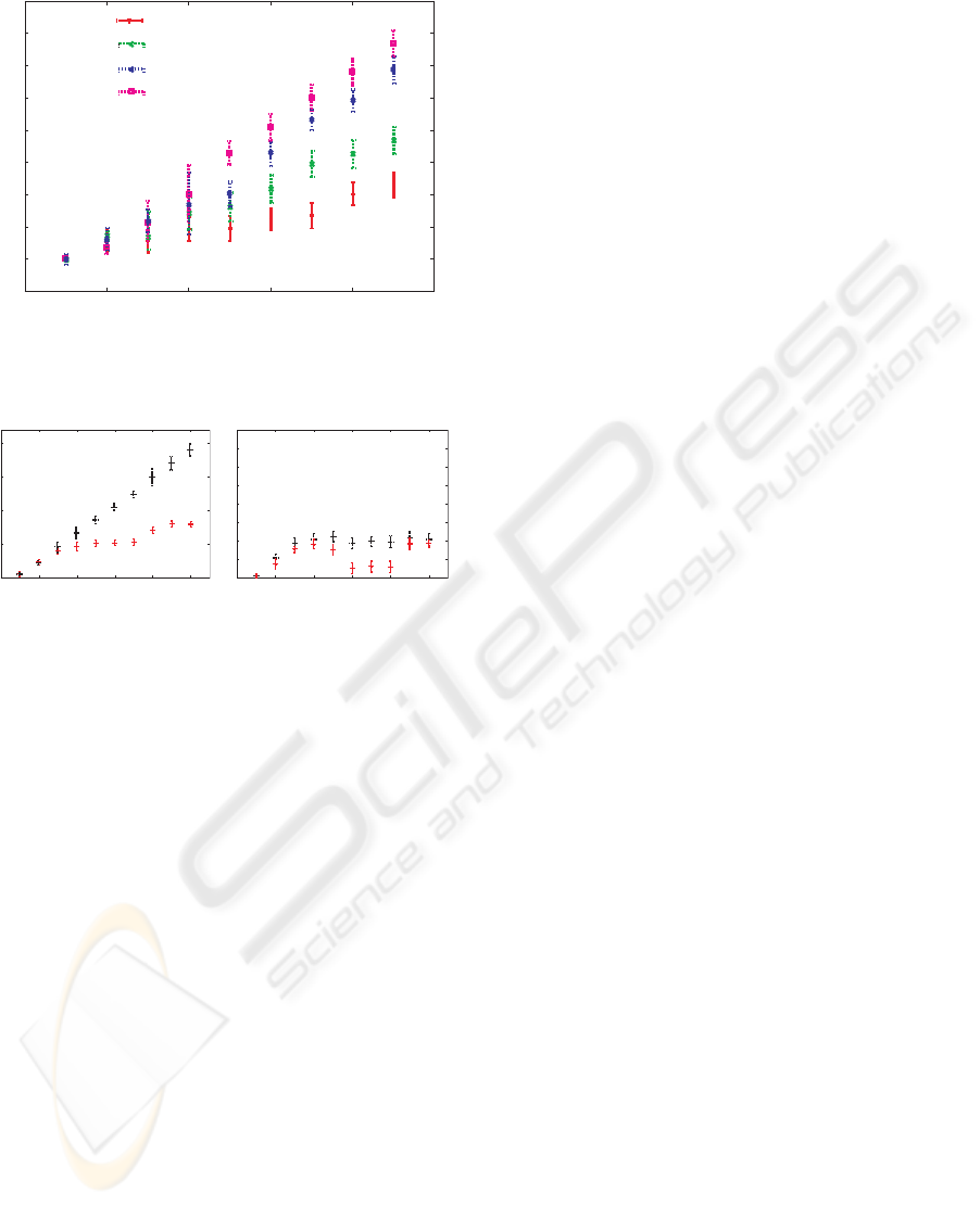
Next, we evaluated the number of frames to which
the local bundle adjustment should be applied. In
other words, we evaluated the relationship between
estimation errors and the number of frames for ap-
plying the local bundle adjustment and identified the
optimal number under the criterion of reducing es-
timation errors most effectively. For the cases of
3 ≤ n ≤ 10, we conducted experiments under the
same condition as described above. We generated 10
steps of motion here. We note that since we have al-
ICINCO 2006 - ROBOTICS AND AUTOMATION
422
-0 .2
0
0 .2
0 .4
0 .6
0 .8
1
1 .2
1 .4
1 .6
3 5 7 9
11
#frames=3
#frames=4
#frames=5
#frames=6
errors
number of steps
Figure 7: The number of frames to which the local bundle
adjustment is applied and estimation errors.
0
0 .5
1
1 .5
2
3 5 7 9 11
0
0 .1
0 .2
0 .3
0 .4
0 .5
0 .6
0 .7
0 .8
3 5 7 9 11
number of steps number of steps
(a) translation vectors (b) rotation matrices
errors
Figure 8: Accumulated errors when the local bundle adjust-
ment with 3 frames is applied (read means with correction
and black means without correction).
ready observed little improvement in accuracy of ro-
tation estimation, we here focused on translation esti-
mation only.
The results for the cases of 3 ≤ n ≤ 6 are illus-
trated in Fig. 7. In each case, we did not conduct mod-
ification until required number of images are obtained
for the bundle adjustment. For example, in the case of
n = 5, the bundle adjustment was applied only after
the 4th step of motion.
Figure 7 shows that estimation accuracy is best in
the case of n = 3. Though we might expect that esti-
mation accuracy increases with the number of images
to which the bundle adjustment is applied, it is not
true. This is because when the number of images is
large, accumulation of estimation errors incurred by
that time already becomes sufficiently large and the
constraints imposed for the modification is not reli-
able any more. We thus observe that the amount of
accumulated errors is too large to significantly reduce.
This discussion is supported by the fact that the case
of n = 3 is most effective. Accordingly, we have to
apply the bundle adjustment by the time when accu-
mulated errors of estimation does not become large.
We now know that three frames are most effective
to apply the bundle adjustment. We next evaluated
how accumulated errors increase depending on the
number of steps of motion in the case of n = 3. We
conducted the experiment here under the same con-
dition above. We note that 11 steps of motion were
generated here.
The results are shown in Fig. 8. We also conducted
the same experiments using the comparison method.
As for rotation estimation, we do not observe any sig-
nificant accumulation of errors for the both methods.
On the other hand, we easily see that from Fig. 8 (a),
accumulation of estimation errors linearly increases
with the number of steps for the comparison method
while that for the proposed method does not; we see
drastic improvement. We may thus conclude that our
method keeps estimation accuracy stable even for a
long trajectory.
4.2 Trajectory Estimation Using
Real Images
We employed the proposed method to estimate an
ego-motion trajectory in the real situation. We also
employed the comparison method to see the effective-
ness of the proposed method.
We used two off-the-shelf cameras (EVI-G20 from
Sony) as active cameras and set up the cameras on the
stage of a tripod so that the baseline distance the two
cameras is about 20cm and the distance of two fixa-
tion points is between 2m and 3m (Fig.9). We assume
that the optical axis of each camera is parallel with the
Z axis of its camera coordinate system and the world
coordinate system is identical with the right-camera
coordinate system at the initial position. We then es-
timated a motion trajectory of the projection center of
the right camera.
We moved the tripod with the cameras in the scene.
The trajectory of the right-camera motion is shown in
Fig.10. The length of the trajectory was about 5m.
We marked 135 points (20 points along each straight
line segment and 45 points along each circular seg-
ment) on the trajectory and regarded them as samples
during the ego motion. (In other words, 135 points
were sampled during the ego motion of about 5m.)
We then applied the proposed method and the com-
parison method respectively only to the samples, i.e.,
the marked points, to estimate the ego motion. We
note that in each method, we selected 3 points from
each right image and 3 points from each left image
and computed the optical-flow vectors of the 6 points
for subsequent computations.
In each image captured by each camera at the start-
ing point of the motion, we manually selected a point
to serve as the fixation point. During the estimation,
we updated fixation points 7 times for each camera in
the case where the current fixation point disappears
from the image. This updating was also conducted by
REDUCING ACCUMULATED ERRORS IN EGO-MOTION ESTIMATION USING LOCAL BUNDLE ADJUSTMENT
423
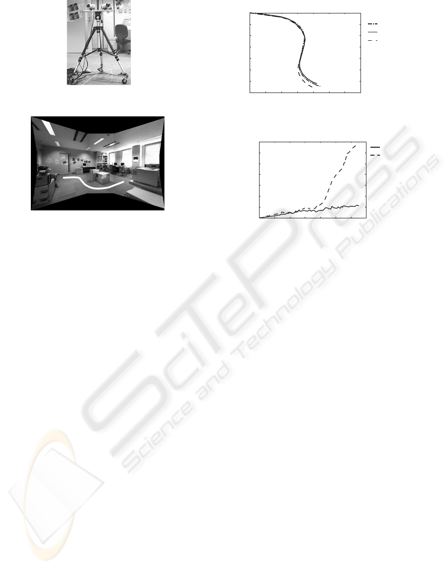
Figure 9: Two camera setup.
Figure 10: Experimental environment.
hand. We computed optical flows within the window
of 100 × 100 pixels whose center is the image of the
fixation point. We used three optical-flow vectors for
each camera (we thus used six optical-flow vectors in
total). The vectors were randomly selected within the
windows of 30 × 30 pixels whose center is the im-
age of the fixation point. In computing optical flows,
we used the Kanade-Lucas-Tomasi algorithm (Lucas
and Kanade, 1981; Tomasi and Kanade, 1991). In the
proposed method, we independently applied the local
bundle adjustment to each camera images where last
three frames with their fixation points are used.
Under the above conditions, we estimated the right-
camera motion at each marked point. The trajectory
of the right-camera motion was obtained by concate-
nating the estimated motions at the marked points.
Fig.11 shows the estimated trajectory that is pro-
jected on the XZ-plane of the world coordinate sys-
tem. Fig. 12 shows errors in position estimation in
each step for the proposed method and for the com-
parison method. In Figs. 11, 12, the solid line and
the dotted line respectively indicate the result by the
proposed method and that by the comparison method.
The broken dotted line in Fig. 11, on the other hand,
indicates the ground truth. Table1 shows the average
and the standard deviation of errors in position esti-
mation over the marked 130 points.
Figure 11 shows that the proposed method more ac-
curately estimates the trajectory than the comparison
method. We observe that from Fig. 12 the compari-
son method fails in estimation around the 80th step
(the beginning of the second circular part of the tra-
jectory) and begins to have aberration from the actual
-350
-300
-250
-200
-150
-100
-50
0
0 50 100 150 200 250 300 350
ground truth
after modification
before modification
Z
cm
X
cm
Figure 11: Estimated camera positions.
0
5
10
15
20
25
30
35
0 20 40 60 80 100 120 140
error
(cm)
step
after modification
before modification
Figure 12: Estimation errors of the camera position.
trajectory. The proposed method, on the other hand,
succeeds in reducing estimation errors incurred in the
step and, as a result, keeps accurate and stable estima-
tions of the subsequent trajectory. The position error
at the terminal marked point was about 35cm for the
comparison method and about 4cm for the proposed
method. We see that estimation accuracy is greatly
improved and that this improvement leads to reducing
accumulation of estimation errors. Table 1 also vali-
dates the effectiveness of the proposed method; not
only the average of estimation errors in each step but
also the standard deviation becomes the smaller. We
can thus conclude that the proposed method realizes
accurate and stable ego-motion estimation even for a
long trajectory.
5 CONCLUSION
The ego-motion estimation method using the binoc-
ular independent fixation control (Sugimoto et al.,
2004; Sugimoto and Ikeda, 2004) involves a problem
that estimation accuracy gradually becomes worse as
the motion trajectory becomes longer and longer be-
cause of accumulation of errors incurred in each es-
timation step. To avoid falling in such a problem,
we proposed a method that incorporates incremen-
tal modification of estimated parameters. Namely,
the proposed method applies the bundle adjustment
in each step only to last several frames so that geo-
metrical consistency, i.e., the epipolar constraint, be-
tween the last frames and the fixation points is guar-
ICINCO 2006 - ROBOTICS AND AUTOMATION
424

Table 1: The average and the standard deviation of estima-
tion errors over 130 steps.
before after
modification modification
average [cm] 0.268 0.0394
standard
deviation [cm] 0.102 0.00739
anteed. With this modification, errors involved in the
parameters before the modification are drastically re-
duced and, therefore, significant improvement of ac-
curacy in estimation for a long trajectory is realized,
with keeping the method incremental.
The proposed method focuses on the fixation point
for evaluating geometrical consistency, however, us-
ing other feature points together may improve estima-
tion accuracy further. An adaptive application of the
bundle adjustment, i,e., effectively selecting steps to
which the local bundle adjustment is applied, will be
promising to reduce computational cost. These inves-
tigations are our future direction.
ACKNOWLEDGEMENTS
This work is in part supported by Grant-in-Aid for
Scientific Research of the Ministry of Education, Cul-
ture, Sports, Science and Technology of Japan under
the contract of 13224051 and 18049046.
REFERENCES
H. Aoki, B. Schiele and A. Pentland (2000): Realtime Per-
sonal Positioning System for Wearable Computers, Vi-
sion and Modeling Technical Report, TR-520, Media
Lab. MIT.
B. Clarkson, K. Mase and A. Pentland (2000): Recognizing
User’s Context from Wearable Sensors: Baseline Sys-
tem, Vision and Modeling Technical Report, Vismod
TR-519, Media Lab. MIT.
A. J. Davison, W. W. Mayol and D. W. Murray (2003):
Real-Time Localization and Mapping with Wearable
Active Vision, Proc. of ISMAR, pp. 18–27.
A. J. Davison and D. W. Murray (1998): Mobile Robot Lo-
calization using Active Vision, Proc. of ECCV, Vol. 2,
pp. 809–825.
G. N. DeSouza and A. C. Kak (2002): Vision for Mobile
Robot Navigation: A Survey, IEEE Trans. on PAMI,
Vol. 24, No. 2, pp. 237–267.
M. W. M. G. Dissanayake, P. Newman, S. Clark, H. F.
Durrant-Whyte and M. Csorba (2001): A Solution
to the Simultaneous Localization and Map Building
(SLAM) Problem, IEEE Trans. on RA, Vol. 17, No. 3,
pp. 229–241.
N. Gonc¸alves and H. Ara
´
ujo (2002): Estimation of 3D Mo-
tion from Stereo Images, Proc. of ICPR, Vol. I, pp.
335–338.
J. E. Guivant and E. Nebot (2001): Optimization of the
Simultaneous Localization and Map-Building Algo-
rithm for Real-Time Implementation, IEEE Trans. on
RA, Vol. 17, No. 3, pp. 242–257.
R. Hartley and A. Zisserman (2000): Multiple View Geom-
etry in Computer Vision, Cambridge Univ. Press.
B. D. Lucas and T. Kanade (1981): An Iterative Image Reg-
istration Technique with an Application to Stereo Vi-
sion, Proc. of IJCAI, pp. 674–679.
N. Molton and M. Brady (2003): Practical Structure and
Motion from Stereo When motion is Unconstrained,
Int. J. of Computer Vision, Vol. 39, No. 1, pp. 5–23.
T. Nakagawa, T. Okatani and K. Deguchi (2004): Active
Construction of 3D Map in Robot by Combining Mo-
tion and Perceived Images, Proc. of ACCV, vol. 1, pp.
563–568.
A. Sugimoto, W. Nagatomo and T. Matsuyama (2004): Es-
timating Ego Motion by Fixation Control of Mounted
Active Cameras, Proc. of ACCV, pp. 67–72.
A. Sugimoto and T. Ikeda (2004): Diverging Viewing-Lines
in Binocular Vision: A Method for Estimating Ego
Motion by Mounted Active Cameras, Proc. of the 5th
Workshop on Omnidirectional Vision, Camera Net-
works and Non-classical Cameras, pp. 67–78.
Y. Sumi, Y. Ishiyama and F. Tomita (2004): 3D Localiza-
tion of Moving Free-Form Objects in Cluttered Envi-
ronments, Proc. of ACCV, vol. 1, pp. 43-48.
S. Thrun (2002): Robotic Mapping: A Survey, Exploring
Artificial Intelligence in the New Millennium, Morgan
Kaufmann.
C. Tomasi and T. Kanade (1991): Detection and Tracking
of Point Features, CMU Technical Report, CMU-CS-
91-132.
B. Triggs, P. McLauchlan, R. Hartley and A. Fitzgibbon
(2000): Bundle Adjustment – A Modern Synthesis,
Vision Algorithms: Theory and Practice (B. Triggs, A.
Zisserman and R. Szeliski eds.) LNCS, Vol. 1883, pp.
298–372, Springer.
B. L. Welch (1938): The Significance of the Difference be-
tween Two Means when the Population Variances are
Unequal, Biometrika, Vol. 29, pp. 350–362.
M. Werman, S. Banerjee, S. Dutta Roy and M. Qiu (1999):
Robot Localization Using Uncalibrated Camera In-
variants, Proc. of CVPR, Vol. II, pp. 353–359.
Z. Zhang and Y. Shan (2001): Incremental Motion Estima-
tion through Local Bundle Adjustment, Technical Re-
port MSR-TR-01-54, Microsoft Research.
Z. Zhang and Y. Shan (2003): Incremental Motion Esti-
mation through Modified Bundle Adjustment, Proc.
ICIP, Vol.II, pp.343–346.
REDUCING ACCUMULATED ERRORS IN EGO-MOTION ESTIMATION USING LOCAL BUNDLE ADJUSTMENT
425
