
TOWARDS A SLAM SOLUTION FOR A ROBOTIC AIRSHIP
Cesar Castro, Samuel Bueno
Computer Vision and Robotics Division, CenPRA
Rod. SP 65, km 143.6, 13069-901, Campinas-SP, Brazil
Alessandro Victorino
INRIA-Sophia Antipolis, ICARE project
2004, Route des Lucioles, 06902, Sophia Antipolis , France
Keywords:
SLAM, localization, mapping, Kalman filtering, UAVs.
Abstract:
This article presents the authors ongoing work towards a six degrees of freedom simultaneous localization and
mapping (SLAM) solution for the Project AURORA autonomous robotic airship. While the vehicle’s mission
is being executed in an unknown environment, where neither predefined maps nor satellite help are available,
the airship has to use nothing but its own onboard sensors to capture information from its surroundings and
from itself, locating itself and building a map of the environment it navigates. To achieve this goal, the airship
sensorial input is provided by an inertial measurement unit (IMU), whereas a single onboard camera detects
features of interest in the environment, such as landmark information. The data from both sensors are then
fused using an architecture based on an extended Kalman filter, which acts as an estimator of the robot pose
and the map. The proposed methodology is validated in a simulation environment, composed of virtual sensors
and the aerial platform simulator of the AURORA project based on a realistic dynamic model. The results are
hereby reported.
1 INTRODUCTION
Beside their use as military surveillance platforms,
Unmanned Aerial Vehicles (UAVs) have a wide spec-
trum of potential civilian observation and data acqui-
sition applications. Usually, unmanned aerial plat-
forms are airplanes, helicopters or, more recently, air-
ships - also known as lighter-than-air (LTA) vehicles.
Unmanned airships have extended airborne capa-
bilities and large payload to weight ratio. They are
therefore best suited for low altitude, low speed or
hovering airborne data gathering missions, where the
vehicle should also take-off and land vertically (Elfes
et al., 1998). In this context, Project AURORA –
Autonomous Unmanned Remote mOnitoring Robotic
Airship – was proposed, aiming the gradual estab-
lishment of the technologies required for autonomous
operation of unmanned robotic airships (Elfes et al.,
1998; Bueno et al., 2002). Presently, AURORA LTA
robotic platform consists of (de Paiva et al., 2006):
i) a 10.5 m long, 34 m
3
of volume and 10 Kg pay-
load capacity nonrigid airship; ii) an onboard sys-
tem containing a PC/104 CPU with RT Linux, sen-
sors and actuators; iii) a portable PC with RT Linux
ground station for system operation; iv) a communi-
cation system comprising radio modems, analogical
and short range wireless Ethernet video links. The
onboard sensor package mainly includes: a GPS, an
Inertial Measurement Unit (IMU), a single firewire
IEEE 1394 digital camera and a Wind sensor. Exper-
imental results achieved so far include path following
flight through a set of pre-defined way points under
lateral and longitudinal control; experimental valida-
tion of visual servoing line following strategies are
under way.
Other important research efforts on robotic air-
ships are described in (Kantor et al., 2001; Wimmer
et al., 2002; Hygounenc et al., 2004) and, consider-
ing Planetary Exploration missions, in (Elfes et al.,
2003). Unmanned LTA vehicles are also suited for
stratospheric HALE (High Altitude Long Endurance)
operation, and efforts in this sense have been carried
out in Japan, Korea, Europe and USA, involving in-
dustry and academia.
For UAVs in general, and for AURORA in particu-
lar, an important aspect of the aircraft embedded sys-
tem is to determine the aerial platform position and
orientation in space. To do so, the most common ap-
proach is to use an inertial navigation system (INS) or
external navigational aids (such as a GPS). However,
241
Castro C., Bueno S. and Victorino A. (2006).
TOWARDS A SLAM SOLUTION FOR A ROBOTIC AIRSHIP.
In Proceedings of the Third International Conference on Informatics in Control, Automation and Robotics, pages 241-248
DOI: 10.5220/0001213202410248
Copyright
c
SciTePress
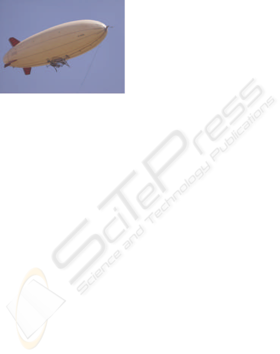
Figure 1: The AURORA project robotic aerial platform.
inertial systems diverge over time and GPS informa-
tion might not always be available. Besides, neither
inertial navigation nor satellite systems provide infor-
mation about the surroundings of the airship, which
means localization with respect to the environment is
not possible. So, more important than finding the pose
of the vehicle is to do so autonomously, using nothing
but its embedded sensors, with no external sensors, no
predefined maps or satellite help. Furthermore, local-
ization in an unknown environment implies not only
pose determination but also incremental map build-
ing. The process in which a mobile robot constructs
a map and, while doing it, locates itself in it, is called
Simultaneous Localization And Mapping (SLAM).
Robotic mapping started with approaches based on
occupancy grids (Elfes, 1987; Elfes, 1989), but it
was only with the work of Smith, Self and Cheese-
man (Smith et al., 1987; Smith et al., 1988) simul-
taneous localization and mapping was first formu-
lated as a probabilistic estimation problem. Since
then, interest in SLAM increased and several tech-
niques were developed, taking the extended Kalman
filter (EKF) approach further (Castellanos et al., 1999;
Castellanos et al., 2001). From the indoors robotics
research community, these solutions were then taken
to open spaces, where the size of the environment
and of the map became a concern (Sukkarieh et al.,
1999; Guivant and Nebot, 2001; Bailey, 2002; Guiv-
ant and Nebot, 2003). Finally, it reached aerial ro-
bots. Some interesting solutions to the SLAM prob-
lem have been posed at the international aerial robot-
ics community, consisting of directly correcting the
IMU readings with the aid of a GPS (Panzieri et al.,
2002) and/or updating the prediction by integrating
the inertial navigation data with observations of the
environment (made by an exteroceptive sensor such as
a range finder or a camera). The aerial SLAM prob-
lem has received relevant attention from the robotic
community over the last years (Ruiz et al., 2001; Kim,
2004; Langelaan and Rock, 2005; Wu et al., 2005)
but, even though many advances and partial solutions
have been proposed, it remains an open problem when
related to autonomous aerial navigation in unknown
and unstructured environments.
Considering the present status of Project AU-
RORA, in this article we present a first effort towards
the establishment of a 3D SLAM solution, with six
degrees of freedom (DoF), specifically aiming to en-
hance the autonomous capability of the robotic air-
ship. An IMU is used in an inertial navigation model
to calculate the displacement of the airship during a
time interval, while a vision system, in which a single
onboard camera is used to capture landmark informa-
tion from the environment, allows the computation of
the map and of the airship pose with respect to it. An
EKF is used to fuse all the information and calculate
the uncertainty of the estimation.
After this introductory section, the remaining parts
of this article are organized as follows. Section 2
describes the methodology used to achieve SLAM
through an extended Kalman filter. Section 3 shows
the simulation results of the methodology. Finally,
Section 4 stresses the concluding remarks and the
future work concerning the implementation of such
methodology on the real airship and its evolution.
2 SYSTEM DESCRIPTION
In this section, the mathematical formulation of the
problem is derived. The Kalman filtering approach to
sensor fusion and autonomous localization and map-
ping is presented, along with the equations that de-
fine the airship movement and the observation model,
which will lead to feature matching and state augmen-
tation.
2.1 SLAM Architecture
Suppose that the airship is placed in an unknown lo-
cation, with no prior information about its surround-
ings. It is equipped with an IMU, which provides roll,
pitch and yaw velocities as well as linear accelera-
tions in the body reference frame, and a single cam-
era, which can be used to take relative measurements
between features in the environment (their absolute
locations are not known) and the camera itself. Usu-
ally, the IMU readings are fed to the inertial naviga-
tion system (INS) of the airship that computes the rel-
ative displacement of the vehicle in a geodesic refer-
ence frame. In the present work, as the vehicle moves
around, features are observed by the camera and fused
to the IMU data in order to build a map and minimize
localization errors of both vehicle and map features.
ICINCO 2006 - ROBOTICS AND AUTOMATION
242

The INS equations are inserted in the vehicle kine-
matic model.
An extended Kalman filter (EKF) is used as a state
estimator for both the vehicle location and the map,
propagating first-order uncertainty, in an approach
known as Stochastic Mapping(Smith et al., 1987;
Smith et al., 1988). For a map with N features, the
system state vector
ˆ
x is defined as the estimate of the
vehicle state vector
ˆ
x
v
augmented with the map state
vector
ˆ
x
m
, so that
ˆ
x =
ˆ
x
v
ˆ
x
m1
.
.
.
ˆ
x
mN
. (1)
The state vector is accompanied by a covariance
matrix P, which represents the uncertainty in the state
vector, defined as
P =
P
v,v
P
v,m1
. . . P
v,mN
P
m1,v
P
m1,m1
. . . P
m1,mN
.
.
.
.
.
.
.
.
.
.
.
.
P
mN,v
P
mN,m1
. . . P
mN,mN
.
(2)
In the following sections, the kinematic model of
the airship using the IMU inputs is derived, along with
the observation model. In the estimation process, the
kinematic model is used to predict the airship pose
and estimate the increase in the pose uncertainty. The
observation model is used to update the previous pre-
diction and reduce the uncertainty of the estimation
based in the observations.
2.2 Kinematic Model
The vehicle state vector is defined as
ˆ
x
v
=
"
ˆ
p
ˆ
v
ˆ
q
#
(3)
where vectors
ˆ
p and
ˆ
v are, respectively, the position
and the velocity of the airship in earth reference. The
orientation of the robot is represented by the quater-
nion vector
ˆ
q. Although it’s a non-mimimal represen-
tation of orientation, a quaternion is used in order to
avoid linearization problems and singularities of other
representations.
The prediction of the robot state
ˆ
x(k|k − 1) is ob-
tained from its last pose and the signals provided by
the IMU that constitute the input u(k) of the inertial
navigation model, composed of: f , the linear accel-
eration, and ω, the angular velocity, both in frame of
reference fixed in the airship:
ˆ
x
v
(k|k − 1) = f(
ˆ
x
v
(k), u(k), w
v
(k))
=
"
ˆ
p(k − 1)
ˆ
v(k − 1)
ˆ
q(k − 1)
#
+
"
∆p
∆v
∆q
#
+
"
w
p
(k)
w
v
(k)
w
q
(k)
#
, (4)
where w(k) represents uncorrelated, zero-mean
process noise errors with covariance Q(k) and
"
∆p
∆v
∆q
#
=
v(k − 1)t + C
W
B
f
t
2
2
C
W
B
f t
(
1
2
D ω + ε q(k − 1)) t
, (5)
D =
q
i
q
j
q
k
−q
r
q
k
−q
j
−q
k
−q
r
q
i
q
j
−q
i
−q
r
, (6)
ε = 1 − kq(k − 1)k
2
. (7)
It is important to notice that C
W
B
is the direction co-
sine matrix obtained from
ˆ
q(k − 1), which takes from
the airship reference frame (B) orientation to the earth
reference frame (W ) orientation, D is also computed
from
ˆ
q(k − 1), and ε represents an integration correc-
tion gain, which comes into place if the norm of the
quaternion is different than one.
2.3 Observation Model
It is important to investigate how the observations of
the landmarks relate to its actual position. In this
work, it is considered that the visual sensor returns to
the system the relative position between camera and
landmark, as shown in figure 2.
Each map feature is represented by its cartesian
threedimensional coordinates in the earth-fixed frame
W , while the observations consist of the cartesian
threedimensional coordinates of the features in the
camera-fixed frame C. Considering the camera frame
to be a known rotation of the airship body frame B, it
is possible to specify each a map feature as
x
mi
= g(x
v
, z
i
)
= p(k) + R
W
B
(R
B
C
(z
i
)), (8)
where R
B
C
(·) is a function that uses a quaternion to
rotate from the camera orientation to the body ori-
entation (the airship orientation) and R
W
B
(·) rotates
a vector from the body frame to the world frame.
Taking the inverse of the previous equation, the ob-
servations at any instant can be predicted from the
state vector with the resulting observation model:
ˆ
z
i
= h(x
v
, x
mi
) + v
i
(k)
= g
−1
(x
v
, x
mi
) + v
i
(k)
= R
C
B
(R
B
W
(x
mi
− p)) + v
i
(k), (9)
TOWARDS A SLAM SOLUTION FOR A ROBOTIC AIRSHIP
243
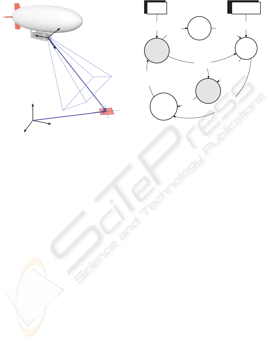
z
i
W
x
mi
C
Figure 2: The airship observing a landmark.
with the rotation functions following the same nota-
tion already specified and v
i
(k) being uncorrelated,
zero mean observation noise with covariance R(k).
2.4 Estimation Process
The general state estimation process using the ex-
tended Kalman filter is represented in Fig. 3. At the
kth step, the kinematic model of the robot is used,
along with the inputs from the IMU, to compute a
prediction
ˆ
x(k|k − 1) and the covariance P(k|k − 1).
Because the IMU readings do not contain any map in-
formation, the uncertainty in the inputs is reflected in
the vehicle state uncertainty, which should increase.
An observation prediction h(
ˆ
x(k|k − 1)) is then cal-
culated and compared to the real observation z(k),
obtained from the vision system. From that compar-
ison, the observations are divided into matched and
unmatched observations. The first are used to gener-
ate the estimate
ˆ
x(k|k) and P(k|k) (the uncertainty
should decrease, since the pose with respect to the
map can be corrected), while the second are used to
augment the state vector and the associated covari-
ance matrix with new map entrances.
2.4.1 Prediction
The prediction of the state vector is obtained directly
from (4), derived in section 2.2. Because the map is
considered static with respect to the earth frame, the
map transition equation is
ˆ
x
m
(k|k − 1) =
ˆ
x
m
(k − 1), (10)
Vision System
(EKF )
predict
(EKF )
update
predict
obs
augment
match
obs
matched
observations
unmatched
observations
xa
(
k
|
k
)
Pa(
k
|
k
)
a(
k
)
w
(
k
)
z
(
k
)
x(
k
|
k
-1)
h(x(
k
|
k
-1))
x(
k
|
k
-1)
P(
k
|
k
-1)
x(
k
|
k
)
P(
k
|
k
)
IMU
Figure 3: Structure of the SLAM system.
which leads to the full state transition equation:
ˆ
x
v
(k|k − 1)
ˆ
x
m
(k|k − 1)
=
f(
ˆ
x
v
(k − 1), u(k), 0)
ˆ
x
m
(k − 1)
(11)
However, as it was already mentioned, the predic-
tion implies an increase of the airship pose uncer-
tainty, since the IMU readings contain errors. There-
fore, the covariance matrix must be recalculated to re-
flect that change. This is done through the following
equation:
P(k|k − 1) = ∇f
x
P(k − 1) ∇f
T
x
+∇f
u
Q(k) ∇f
T
u
, (12)
in which ∇f
x
and ∇f
u
are the jacobians of f with
respect to the state vector and the input, respectively.
The diagonal matrix Q(k) represents a model of the
error covariance in the sensor readings.
2.4.2 Update
In order to update the prediction x(k|k − 1), using the
landmarks perceived by the vision system, the equa-
tions derived in section 2.3 are used. From (9), it is
possible to calculate the uncertainty in the observa-
tion prediction at instant k, S(k), which is related to
the system state and the observation errors:
S(k) = ∇h
x
(k)P(k|k − 1)∇h
T
x
(k) + R(k), (13)
where ∇h
x
(k) is the Jacobian of h(x) with respect to
ˆ
x(k|k − 1) and R(k) is the sensor uncertainty, mod-
eled as a diagonal matrix.
From (9) and (13), the observations are associated
to their predictions in observation space. A statistical
ICINCO 2006 - ROBOTICS AND AUTOMATION
244

validation gate, the Mahalanobis distance, is used to
match observations. This distance γ is computed by
γ
i,j
= ν
T
i,j
S
−1
j
(k) ν
i,j
, (14)
where S
j
(k) is the covariance related to the jth pre-
diction and ν
i,j
is the innovation vector, defined as
ν
i,j
= z
i
− h(
ˆ
x
v
,
ˆ
x
mj
). (15)
If any prediction or observation is matched twice, it is
necessary to resolve the ambiguity. The method used
in the present work is the nearest neighbors data as-
sociation, in which the observation is matched against
the prediction with the smallest value N
i,j
,
N
i,j
= γ
i,j
+ ln |S
j
(k)|. (16)
If any match is found, not only the state is updated
but the uncertainty in both airship position and map
can be reduced, according to the following:
ˆ
x(k) =
ˆ
x(k|k − 1) + W(k)ν(k), (17)
P(k) = P(k|k − 1)
−W(k)S(k)W(k)
T
, (18)
where ν(k) is calculated from the union of the
matched predictions and observations, the gain ma-
trix W(k) is obtained from
W(k) = P(k|k − 1)∇h
T
x
(k)S
−1
(k) (19)
and S(k) is computed as in (13).
2.4.3 State Augmentation
The unmatched features must be included in the map,
in order for them to be used in the update stage the
next time they are observed. The process of incremen-
tally building the map is known as state augmentation
and is accomplished by the following equation:
x
aug
(k) = f
a
(x(k)) =
"
x
v
(k)
x
m
(k)
g(x
v
(k), z(k))
#
, (20)
with g(·, ·) defined in (8). The newly added map fea-
ture is highly correlated to the vehicle state, due to the
fact that position and orientation uncertainty directly
affect the new landmark uncertainty. To accommo-
date that situation, the matrix P(k) must change ac-
cordingly:
P
aug
(k) = ∇f
a
P(k) 0
0 R(k)
∇f
T
a
(21)
With these equations, the cycle shown in figure 3
was fully described.
3 RESULTS
In this section, the described methodology is vali-
dated in simulation. The simulation setup and the per-
formance measurements are presented, as well as an
analysis of the results.
3.1 Simulation Setup
The SLAM implementation and studies reported here
were done in a simulation environment for the AS800
airship (Gomes and Ramos, 1998; de Paiva et al.,
1999). In the simulator, the airship 6DoF dynamics
are modeled according to
M
˙
v = F
d
(v) + F
a
(v) + F
p
+ F
g
, (22)
where M is the mass matrix which includes both the
actual inertia of the airship and the virtual inertia ele-
ments associated with the dynamics of buoyant vehi-
cles; v = [ u, v, w, p, q, r ]
T
is the vector of the air-
ship linear and angular velocities; F
d
is the dynamics
vector containing the Coriolis and centrifugal force
terms, and also the wind-induced forces (Azinheira
et al., 2001); F
a
is the vector of aerodynamic forces
and moments; F
p
is the vector of propulsion forces
and moments, and F
g
represents the gravity forces
and moments.
In order to test the SLAM scheme in different con-
ditions during the simulated flight, the airship is ex-
posed to mild wind and turbulence, also experiencing
different accelerations and turns. Lateral and longitu-
dinal control schemes are used to make the airship fol-
low a trajectory path defined as a sequence of straight
lines between a set of pre-defined points in latitude,
longitude and altitude. The lateral heading/guidance
control uses a PID controller as described in (Azin-
heira et al., 2000). The longitudinal control involves
an altitude state feedback controller with a propor-
tional plus derivative (PD) action, and a simple pro-
portional velocity controller (Bueno et al., 2002).
Virtual implementations of an IMU and a vision
system were developed so that the SLAM algorithms
could be effectively tested. The virtual IMU consists
simply of a module that collects the IMU perfect read-
ings, which are used to describe the error free path of
the airship, and adds a noise with the selected distri-
bution. The virtual vision system includes the simu-
lation of a camera, comprising focus, aspect and the
direction axes (which can be modified to reflect me-
chanical imperfections). With these parameters, im-
ages of the environment can be rendered in a visual-
ization frontend, as shown in Fig. 4. Also, it calcu-
lates the observations based in the environment math-
ematical representation, emulating an algorithm that
can return the relative position of the map landmarks
with respect to the camera. To this relative position, it
adds an error with known distribution to reflect other
noise sources.
Before starting the simulation, the airship is placed
at an arbitrary position in the virtual 3D world and the
initial estimate is set at the same pose. Because the
estimate and the map are made relative to the initial
setup of the system, the divergence between the real
TOWARDS A SLAM SOLUTION FOR A ROBOTIC AIRSHIP
245
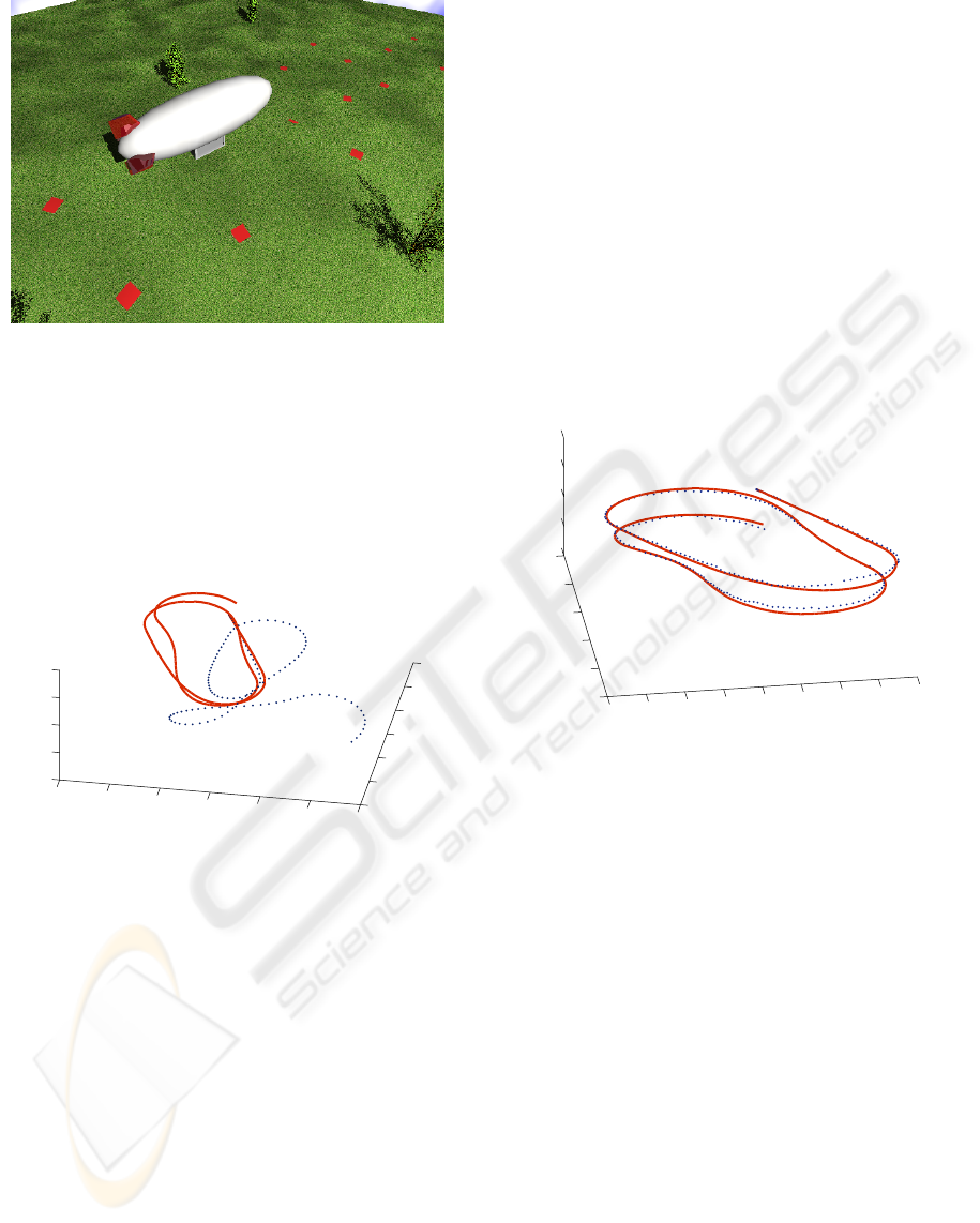
Figure 4: Renderization of the virtual environment, display-
ing the airship in flight and the landmarks on the field.
state of the system and its estimate will directly show
the estimation error.
50
100
150
200
250
300
350
−200
−150
−100
−50
0
50
100
−1000
−500
0
500
1000
y axis
end →
x axis
← start
z axis
Figure 5: Comparison of the real trajectory (solid line) with
the one obtained from the IMU alone (dotted line). The
estimation diverges unconstrained.
As in the real onboard airship infrastructure (Bueno
et al., 2002; de Paiva et al., 2006), in the simulation
environment, new information from the virtual IMU
and vision system are provided every 0.05 seconds
(20 Hz). The IMU readings contain an error with dis-
tribution N (−0.03, 0.04) in m/s
2
in the linear accel-
eration f and N(0.01, 0.0025) rad/s in the angular
velocity ω, which means that both of them lead to a
serious drift that, if not corrected, accumulates over
time, generating ever increasing errors, as it is seen in
Fig. 5. The vision system makes observations of land-
marks (which are unknown to the vehicle system) and
detects their relative position with an additional error
with zero mean and a variance of 2.25 m in each of
the coordinates (x
b
i
, y
b
i
, z
b
i
).
3.2 SLAM System Performance
In what follows, localization and mapping results
of the proposed methodology are presented and dis-
cussed.
In terms of localization, Fig. 6 compares the path
followed by the airship during the experiment and the
trajectory computed by using the SLAM scheme. The
solid line represents the real position of the airship,
while the dotted line represents the estimate of the air-
ship position using the SLAM-EKF methodology. In
contrast to the IMU-only estimate shown in Fig. 5,
the estimation error does not grow indefinitely and is
always small, considering the errors in both the IMU
and the vision system.
80
100
120
140
160
180
200
220
240
−150
−100
−50
0
50
100
20
30
40
50
60
end →
← start
x axis
y axis
z axis
Figure 6: Comparison of the real trajectory (solid line) with
its estimate, using the SLAM methodology (dotted line).
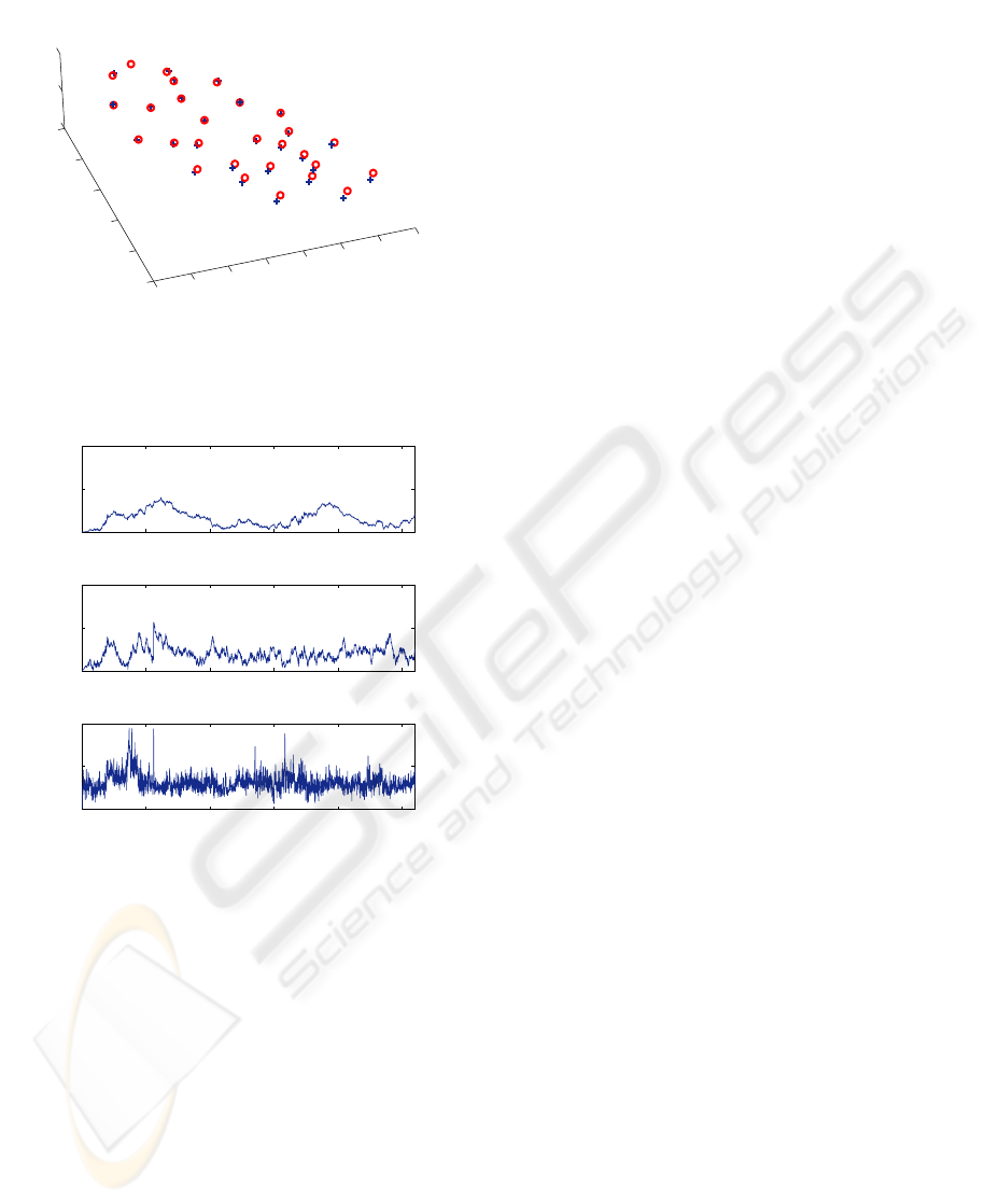
The generated map associated to the previous tra-
jectory is shown in Fig. 7. The circles represent the
position of the real landmarks, while the crosses show
the map estimate. As in the trajectory, the errors are
small. The mean distance from the estimates to the
real landmarks is 2.26 meters and the maximum dis-
tance is 4.59 m.
The error norm of the vehicle state, separated in
position, velocity and orientation, is shown in Fig.
8, and they demonstrate the overall SLAM conver-
gence. To understand the behavior of these errors
during some points of the flight, it is necessary to an-
alyze the number of feature matches at each obser-
vation and the covariance of the map features. With
less than three matched features, the update stage will
not respond properly, as a unique position of the air-
ship with respect to the matched features cannot be
calculated. Also, when there are too many recently
discovered features being observed, their covariance
is high and the gain matrix W will not favor the up-
date, which means very quick turns and high speeds
will stop the system from working properly.
ICINCO 2006 - ROBOTICS AND AUTOMATION
246
0
50
100
150
200
250
300
350
−300
−200
−100
0
100
200
−40
−20
0
x axis
y axis
z axis
Figure 7: Real map, represented by circles, and the esti-
mated map, represented by crosses.
0 500 1000 1500 2000 2500
0
5
10
iteration
ˆ
p error norm
0 500 1000 1500 2000 2500
0
0.5
1
iteration
ˆ
v error norm
0 500 1000 1500 2000 2500
0
0.02
0.04
iteration
ˆ
q error norm
Figure 8: On top is the position error norm. In the middle, it
is shown the velocity error norm. Bellow, is the orientation
quaternion error norm.
It is also important to point out that, even in ideal
conditions, the estimation system is always underde-
termined. If N features are matched, the dimension of
the 6Dof SLAM system is 9+3N, while the observa-
tions can provide rank 6 + 3N . This, however, does
not pose a problem to relative positioning and map-
ping. As the system converges, the errors related to
the landmarks will tend to zero, the airship pose with
respect to the map will be updated to its best and the
position of the landmarks will stop being corrected.
4 CONCLUSION
In this article, a methodology to estimate the AU-
RORA aerial platform position and attitude while in-
crementally building a map of the environment was
derived. A strategy to fuse the data provided by the
airship IMU and the vision system – which detects
the relative position between the landmarks and the
camera – using an extended Kalman filter was pre-
sented. The validation of the proposed methodology
was performed using a realistic simulation environ-
ment that includes the airship dynamic model and au-
tomatic trajectory control used in real flights, a set of
virtual sensors and a visualization frontend.
The obtained results demonstrate the correctness of
the SLAM approach and constitute an important step
in the Project AURORA effort towards the incremen-
tal evolution of robotic airships. Considering the ex-
perimental validation objectives, the SLAM method-
ology hereby presented will be improved and inte-
grated to the airship embedded system for subsequent
experimental validation in real flights. Considering
this objective, further work comprises: i) conclud-
ing the SLAM experiments with the real airship, de-
tecting simple artificial landmarks placed in the en-
vironment; ii) computational performance optimiza-
tions, aiming for larger maps and the simultaneous
observation of many landmarks; iii) a bearing-only
vision system, comprising a landmark tracking algo-
rithm and an efficient feature initialization approach,
which will allow faster computation of the vehicle and
map state update (Davison, 2003); iv) a visual odom-
etry model where the relative motion of the airship
is recovered by decomposing the Euclidean homog-
raphy, established from projective geometry relation-
ships (Silveira et al., 2006).
ACKNOWLEDGEMENTS
The present work was sponsored by the Brazil-
ian agency FAPESP, under grants 04/13467-5 and
03/13845-7. The authors thank Dr. Ely Paiva, for
his support concerning the airship dynamic model and
control strategies, and Dr. Paulo Valente for his assis-
tance regarding Mr. Castro’s M.Sc. work.
REFERENCES
Azinheira, J. R., de Paiva, E. C., Ramos, J. G., Bueno, S. S.,
and Bergerman, M. (2001). Extended dynamic model
for aurora robotic airship. In 14th AIAA Lighter-Than-
Air Systems Technology Conference.
Azinheira, J. R., de Paiva, E. C., Ramos, J. J. G., and
Bueno, S. S. (2000). Mission path following for an
TOWARDS A SLAM SOLUTION FOR A ROBOTIC AIRSHIP
247

autonomous unmanned airship. In International Con-
ference on Robotics and Automation, San Francisco,
USA.
Bailey, T. (2002). Mobile Robot Localisation and Mapping
in Extensive Outdoor Environments. PhD thesis, Aus-
tralian Centre for Field Robotics, University of Syd-
ney.
Bueno, S. S., Azinheira, J. R., Ramos, J. G., de Paiva,
E. C., Rives, P., Elfes, A., Carvalho, J. R. H., and Sil-
veira, G. F. (2002). Project aurora - towards an au-
tonomous robotic airship. In Workshop on Aerial Ro-
botics. IEEE International Conference on Intelligent
Robot and Systems, Lausanne, Switzerland.
Castellanos, J. A., Montiel, J. M. M., Neira, J., and Tards,
J. D. (1999). The spmap: A probabilistic framework
for simultaneous localization and map building. IEEE
Transactions on Robotics and Automation.
Castellanos, J. A., Neira, J., and Tards, J. D. (2001). Mul-
tisensor fusion for simultaneous localization and map
building. IEEE Transactions on Robotics and Automa-
tion.
Davison, A. (2003). Real-time simultaneous localisation
and mapping with a single camera. In Ninth Intl. Con-
ference on Computer Vision.
de Paiva, E. C., Azinheira, J. R., Ramos, J. G., Moutinho,
A., and Bueno, S. S. (2006). Project aurora: in-
frastructure and flight control experiments for a ro-
botic airship. Journal of Field Robotics. In press.
de Paiva, E. C., Bueno, S. S., Gomes, S. B. V., Ramos, J.
J. G., and Bergerman, M. (1999). A control system de-
velopment environment for aurora’s semi-autonomous
robotic airship. In Int. Conference on Robotics and
Automation.
Elfes, A. (1987). Sonal-based real-world mapping and nav-
igation. IEEE Journal of Robotics and Automation.
Elfes, A. (1989). Occupancy Grids: A Probabilistic Frame-
work for Robot Perception and Navigation. PhD the-
sis, Department of Electrical and Computer Engineer-
ing, Carnegie Mellon University.
Elfes, A., Bueno, S. S., Bergerman, M., and Ramos, J. J. G.
(1998). A semi-autonomous robotic airship for envi-
ronmental monitoring missions. In Int. Conf. on Ro-
botics and Automation.
Elfes, A., Bueno, S. S., Bergman, M., de Paiva, E. C.,
Ramos, G. J., and Azinheira, J. R. (2003). Robotic
airships for exploration of planetary bodies with an
atmosphere: Autonomy challenges. Autonomous Ro-
bots.
Gomes, S. B. V. and Ramos, J. J. G. (1998). Airship
dynamic modeling for autonomous operation. In
Int. Conference on Robotics and Automation, Leuven,
Belgium.
Guivant, J. and Nebot, E. (2001). Optimization of the simul-
taneous localization and map-building for real-time
implementation. IEEE Transactions on Robotics and
Automation.
Guivant, J. and Nebot, E. (2003). Solving computational
and memory requirements of feature-based simultane-
ous localization and mapping algorithms. IEEE Trans-
actions on Robotics and Automation.
Hygounenc, E., Jung, I., Soures, P., and Lacroix, S. (2004).
The autonomous blimp project of laas-cnrs: achieve-
ments in flight control and terrain mapping. Intl. Jour-
nal of Robotics Research.
Kantor, G., Wettergreen, D., Ostrowski, J., and Singh, S.
(2001). Collection of environmental data from and air-
ship platform. In SPIE Conference on Sensor Fusion
and Decentralized Control in Robotic Systems IV.
Kim, J. (2004). Autonomous Navigation for Airborne Ap-
plications. PhD thesis, Australian Centre for Field Ro-
botics, University of Sydney.
Langelaan, J. and Rock, S. (2005). Towards autonomous
uav flight in forests. In AIAA Guidance, Navigation
and Control Conference.
Panzieri, S., Pascucci, F., and Ulivi, G. (2002). An out-
door navigation system using gps and inertial plat-
form. IEEE/ASME Transactions on Mechatronics.
Ruiz, I. T., Pelillot, Y., Lane, D. M., and Salson, C. (2001).
Feature extraction and data association for auv con-
current mapping and localisation. In IEEE Interna-
tional Conference on Robotics and Automation.
Silveira, G., Malis, E., and Rives, P. (2006). Visual servo-
ing over unknown, unstructured, large-scale scenes. In
IEEE International Conference on Robotics and Au-
tomation, Orlando, USA.
Smith, R., Self, M., and Cheeseman, P. (1987). A stochas-
tic map for uncertain spatial relationships. In Fourth
International Symposium on Robotics Research.
Smith, R., Self, M., and Cheeseman, P. (1988). Estimat-
ing uncertain spatial relationships in robotics. In Au-
tonomous Robot Vehicles. Springer Verlag.
Sukkarieh, S., Nebot, E., and Durrant-Whyte, H. (1999).
A high integrity imu/gps navigation loop for au-
tonomous land vehicle applications. IEEE Transac-
tions on Robotics and Automation.
Wimmer, D., Bildstein, M., Well, K. H., Schlenker, M.,
Kingl, P., and Krplin, B. (2002). Research airship
”lotte”: development and operation of controllers for
autonomous flight phases. In IEEE/RSJ Int. Confer-
ence on Intelligent Robots and Systems.
Wu, A., Johnson, E., and Proctor, A. (2005). Vision-aided
inertial navigation for flight control. In AIAA Guid-
ance, Navigation and Control Conference.
ICINCO 2006 - ROBOTICS AND AUTOMATION
248
