ROBUST POSTURE CONTROL OF A MOBILEWHEELED
PENDULUM MOVING ON AN INCLINED PLANE
Danielle Sami Nasrallah
1†
, Hannah Michalska
2†
and Jorge Angeles
1†
1
Department of Mechanical Engineering,
2
Department of Electrical and Computer Engineering,
and
†
Centre for Intelligent Machines
McGill University, Montreal, Canada
Keywords:
Wheeled Robots, Nonholonomy, Posture Control, Inclined Plane, Zero-Dynamics, Lyapunov Functions, Slid-
ing Mode, Invariance, Parameters Uncertainties.
Abstract:
The paper considers a specific class of wheeled mobile robots referred to as mobile wheeled pendulums
(MWP). Robots pertaining to this class are composed of two wheels rotating about a central body. The main
feature of the MWP pertains to the central body, which can rotate about the wheel axes. As such motion is
undesirable, the problem of the stabilization of the central body in MWP is crucial. The novelty of the work
presented here resides in the construction of a three-imbricated loop controller that delivers the full control
strategy for the robot posture and copes with parameters uncertainties. Simulations on the performance of the
controlled system are provided.
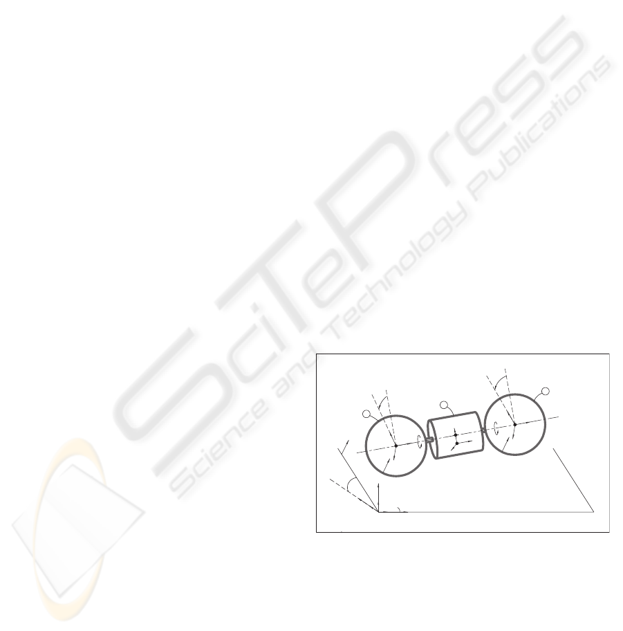
1 INTRODUCTION
This paper introduces a three-loop robust control
scheme for controlling the posture of an anti-tilting
outdoor mobile robot, ATOM, moving on an inclined
plane. ATOM is composed of three rigid bodies: the
central body, a cylinder whose center of mass is offset
from its geometric center, and two spherical wheels
rotating about the central body, as shown in Fig. 1.
The system inputs are the two torques applied to the
wheels. According to its structure, ATOM pertains
to the class of Mobile Wheeled Pendulums (MWP).
Many developments in the field of MWP have been
reported recently: the US patent behind the Gin-
ger and then the Segway Human Transporter projects
(Kamen et al., 1999), JOE, a mobile inverted pendu-
lum (Grassser et al., 2002), and, more recently, Qua-
simoro, a quasiholonomic mobile robot (Salerno and
Angeles, 2004). A feature common to MWPs, that
is not encountered in other wheeled robots, is that
their central body, which constitutes the robot plat-
form, can rotate about the wheels axis. This motion
must not occur, leading to a new challenging prob-
lem for MWP which is the stabilization of the cen-
tral body, aside the classical control problem due to
nonholonomy. Therefore, although an intensive liter-
ature has dealt with the control of wheeled robots in
the past (Campion et al., 1990; Samson and Abder-
rahim, 1999; Astolfi, 1994; Wit and Sordalen, 1992;
Chwa, 2004; Guldner and Utkin, 1994), the control
techniques reported there cannot be applied to MWP
directly.
n
β
θ
13
θ
23
F
0
x
y
z
i
j
k
u
1
v
1
u
2
v
2
u
3
v
3
l
l
l
1
2
3
C
1
C
2
C
3
C
o
P
1
P
2
Figure 1: ATOM robot.
F
or example, any attempt to control the robot mo-
tion in conventional input-output mode results in un-
stable zero-dynamics, unless a friction torque is in-
troduced between the central body and the wheels—
such friction damps naturally the oscillation and elim-
inates trivially the serious issue of unstable zero-
dynamics as it has been the case in (Grassser et
al., 2002; Salerno and Angeles, 2004). (Pathak et
al., 2005) were the first to attempt a solution to the
34
Sami Nasrallah D., Michalska H. and Angeles J. (2006).
ROBUST POSTURE CONTROL OF A MOBILEWHEELED PENDULUM MOVING ON AN INCLINED PLANE.
In Proceedings of the Third International Conference on Informatics in Control, Automation and Robotics, pages 34-41
DOI: 10.5220/0001213100340041
Copyright
c
SciTePress

problem of the unstable zero-dynamics. This was
done by introducing a two-layer controller. How-
ever, such stabilization of the central body is achieved
only locally, i.e., for inclination angles of the central
body near zero, as conventional linearization is em-
ployed. Moreover, the controller proposed there lacks
robustness with respect to parameters uncertainties.
Furthermore, most of the work done in the field of
wheeled robots to date, including the references cited
above, considers robots moving on a horizontal plane.
In the light of previous contributions, the novelty of
the work reported here is as outlined below:
1. To the best of the authors’ knowledge, this is the
first attempt to fully control the posture of a MWP-
class robot moving on an inclined plane.
2. The posture control is achieved simultaneously
with the stabilization of the central body, except
that no restrictions on the central body inclina-
tion are considered, thus rendering the control pro-
posed here global, and solving the unstable zero-
dynamics problem regardless of the central body
inclination. The control is accomplished by using
a three-loop feedback structure with (i) the inner
loop, based on input-output linearization, respon-
sible for the stabilization of the central body and
the control of the steering rate, (ii) the intermedi-
ate loop, based on an intrinsic dynamic property
that is referred to as the natural behavior of the
system, responsible for the control of the heading
velocity, and (iii) the outer loop, based on sliding-
mode control and Lyapunov functions for naviga-
tion, responsible for the posture control. It is note-
worthy that after stabilizing the central body and
controlling heading and steering velocities, the sys-
tem becomes equivalent to any car-like robot, thus
allowing the application of conventional techniques
for position and orientation control. Therefore, the
structure of the external loop is based on the work
reported in (Guldner and Utkin, 1994), with an
additional improvement to ensure smooth entering
into the sliding mode.
3. It is shown that a special choice of the general-
ized coordinates (Euler-Rodrigues parameters, as
opposed to Euler angles used in all the other ref-
erences), combined with a particular selection of
the system output functions in the inner loop, glob-
ally linearizes the dependence between the selected
output variables of the inner loop and the forward
acceleration of the robot. It is this feature that
makes the approach outlined here more powerful
than that of (Grassser et al., 2002; Salerno and An-
geles, 2004; Pathak et al., 2005), as it eliminates
the need to apply local linearization, rendering the
technique completely global and nonlinear. More-
over, this linear dependance allows us to imple-
ment a linear controller for the intermediate loop,
which, combined to the sliding-mode controller of
the outer loop, renders the full control scheme less
sensitive to parameters uncertainties.
The paper is organized in sections 2–4 below. In
Section 2 we formulate the system state-space repre-
sentation. In Section 3 we construct the three-loop
controller. In Section 4 we present the simulation re-
sults confirming the expected performance of the con-
troller.
2 MATHEMATICAL MODEL
The spherical shape of ATOM’s wheels allows the ro-
bot to recover its posture after flipping over, thus ren-
dering it anti-tilting. Moreover, the centers of mass of
the wheels are assumed, by design, to coincide with
the geometric centers of the spheres, while the center
of mass of the central body is offset from its geomet-
ric center. The wheels are denoted bodies 1 and 2,
while the central body is body 3, the symbols used
for the robot modeling being summarized in Table 1.
The Euler-Rodrigues parameters r
0
and r are used to
Table 1: List of Symbols.
b Distance between the wheel centers
c
i
Position vector of the center of mass
C
i
of the i
th
body, i = 1, 2, 3
c
o
Position vector of the geometric center
C
o
of the central body
d Offset between the geometric center
and the center of mass of the central
body
{i, j, k} Right-handed orthogonal triad descri-
bing the orientation of the inertial
frame F
0
l Unit vector along the line of wheel
centers, directed from C
1
to C
2
m
c
Mass of the central body
m
w
Mass of each wheel
n Unit vector normal to the inclined
plane
r
w
Radius of each wheel
r
0
, r Euler-Rodrigues parameters descri-
bing the orientation of the central body
{u
i
, l, v
i
} Right-handed orthogonal triad descri-
bing the orientation of the i
th
body
v
3
Unit vector directed from C
3
to C
o
I
c
Inertia matrix of the central body
I
w
Inertia matrix of each wheel
θ
i3
Angular displacement of the i
th
wheel
with respect to the central body
τ
i
Torque applied to the i
th
wheel
ω
i
Angular velocity vector of the i
th
body in F
0
ROBUST POSTURE CONTROL OF A MOBILEWHEELED PENDULUM MOVING ON AN INCLINED PLANE
35

describe the orientation of body 3 in the inertial frame
F
0
. In our previous work (Nasrallah et al., 2005), the
mathematical model of ATOM moving on a general
warped surface was developed. The terrain geome-
try enters the dynamics explicitly via the vectors nor-
mal to the ground at the contact points. Moreover, the
particular case corresponding to the motion on an in-
clined plane is also included. Furthermore, in a more
recent work (Nasrallah et al., 2006), we performed a
model reduction that facilitates understanding the in-
trinsic dynamic properties of the system. Therefore,
we present below the state-space formulation of the
reduced model.
The six-dimensional vector of generalized coordi-
nates q is defined as
q =
x
c
o
y
c
o
r
T
r
0
T
(1)
while the three-dimensional vector of independent
velocities is
v = [
v
c
ω
3p
ω
3l
]
T
(2)
where v
c
is the heading velocity of the robot,
namely,
v
c
=
r
w
2
(
˙
θ
13
+
˙
θ
23
+ 2ω
3l
)
while ω
3p
is the robot steering rate, given by
ω
3p
=
r
w
b
(
˙
θ
13
−
˙
θ
23
)
and ω
3l
is the projection along the line of (wheels)
centers of ω
3
, the angular velocity of the central body.
The nine-dimensional state vector thus becomes
x
T
=
q
T
v
T
(3)
and the full state-space model of the system is, in
turn,
˙
x = f (x) + g
p
(r
0
, r)τ
p
+ g
m
(r
0
, r)τ
m
(4)
where
f(x) =
v
c
h
T
i
v
c
h
T
j
(1/2)(r
0
1 − R)(ω
3p
n + ω
3l
l)
−(1/2)r
T
(ω
3p
n + ω
3l
l)
f
v
while
g
p
=
0
T
6
g
T
v
p
T
and g
m
=
0
T
6
g
T
v
m
T
with
f
v
=
r
w
(F
b
+ F
c
+ G
b
+ G
c
)
(2r
w
/b)(F
a
+ G
a
)
F
b
+ G
b
and
g
v
p
=
r
w
J
d
0
−J
c
, g
v
m
=
0
(2r
w
/b)J
a
0
Moreover, h is a unit vector given by
h = l × n
while R is the cross-product matrix (CPM)
1
of vector r, and 1 is the 3 × 3 identity matrix.
Furthermore the input torques τ
1
and τ
2
have been
transformed into τ
p
and τ
m
, as follows
τ
p
= τ
1
+ τ
2
and τ
m
= τ
1
− τ
2
(5)
and
F
a
(r
0
, r, v) = J
a
[−4C
d
ω
3p
ω
3l
+ (2/r
w
)C
b
ω
3p
v
c
]
F
b
(r
0
, r, v) = (J
c
− J
b
)(b/r
w
)C
b
(ω
3p
2
+ ω
3l
2
)
+J
b
(b/r
w
)C
d
ω
3p
2
F
c
(r
0
, r, v) = −J
d
(b/r
w
)C
b
(ω
3p
2
+ ω
3l
2
)
−J
c
(b/r
w
)C
d
ω
3p
2
G
a
(r
0
, r) = −2J
a
m
c
g d(r
w
/b)(v
3
× n)
T
k
G
b
(r
0
, r) = (J
c
− J
b
)(2m
w
+ m
c
)g r
w
h
T
k
+J
b
m
c
g d u
T
3
k
G
c
(r
0
, r) = −J
c
m
c
g d u
T
3
k − J
d
(2m
w
+ m
c
)g r
w
h
T
k
C
a
(r
0
, r) = m
c
(r
w
d
2
/b)h
T
u
3
h
T
v
3
C
b
(r
0
, r) = m
c
(r
2
w
d/b)h
T
v
3
C
c
(r
0
, r) = (r
w
/b)(I
cu
− I
cv
)h
T
u
3
h
T
v
3
C
d
(r
0
, r) = C
a
+ C
c
I
a
= 2(r
w
/b)
2
I
wu
+ I
wl
+ m
w
r
2
w
+ m
c
r
2
w
/4
I
b
= −2(r
w
/b)
2
I
wu
+ m
c
r
2
w
/4
I
c
= I
wl
+ m
w
r
2
w
+ m
c
r
2
w
/2
I
d
= I
cl
+ m
c
d
2
I
e
(r
0
, r) = (r
w
/b)
2
[(I
cu
+ m
c
d
2
)h
T
v
3
2
+ I
cv
h
T
u
3
2
]
I
f
(r
0
, r) = m
c
(r
w
d/2)h
T
u
3
J
a
(r
0
, r) = (1/2)/(I
a
− I
b
+ 2I
e
)
J
b
(r
0
, r) = I
c
/(I
c
I
d
− 2I
f
2
)
J
c
(r
0
, r) = (I
c
− I
f
)/(I
c
I
d
− 2I
f
2
)
J
d
(r
0
, r) = (I
d
/2 − I
f
)/(I
c
I
d
− 2I
f
2
)
3 POSTURE CONTROL
In this section we discuss posture control of ATOM
as it moves on an inclined plane. This control objec-
tive must be achieved simultaneously with the stabi-
lization of the central body in order to avoid unstable
zero-dynamics. The controller introduced here has a
triple-loop feedback structure, as shown in Fig. 2. The
task of the inner loop is to control, via the system in-
puts τ
p
and τ
m
, two variables: (i) the steering rate
1
The CPM of a vector v ∈ IR
3
is defined, for every
x ∈ IR
3
as well, as V = CPM(v) = ∂(v × x)/∂x
ICINCO 2006 - ROBOTICS AND AUTOMATION
36
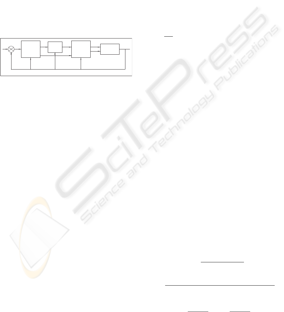
ω
3p
, and (ii) a function of the system outputs. It is
worth noticing that this function is chosen judiciously
in order to stabilize the central body and to provide
a linear dependence with the heading acceleration ˙v
c
.
Then, the task of the intermediate loop is to control
the heading velocity v
c
, while the task of the outer
loop is to control the robot position and orientation
via v
c
and ω
3p
using sliding mode control with Lya-
punov function for navigation. Note that the interme-
diate loop benefits of an intrinsic dynamical property
that is referred to as the natural behavior of the sys-
tem and was introduced in a previous work (Nasrallah
et al., 2006). In the present work, we will employ that
property.
Position
&
Orientation
control
Heading
velocity
control
Central body
oscillation
&
Turning rate
control
ATOM
v
∗
c
ξ
∗
1
ω
∗
3p
τ
p
τ
m
Figure 2: The block diagram of the robot and its associated
control scheme.
The triple-loop controller is designed in sections 1–
6 below. In Section 1 we introduce the normal form
leading to the input-output linearization of the system.
In Section 2 we synthesize the inner-loop. In Section
3 we derive the explicit relation between the heading
acceleration and the output function of the inner loop.
In Section 4 we synthesize the intermediate loop. In
Section 5 we define the Lyapunov function for nav-
igation and the sliding surface that will be used for
posture control and synthesize the outer-loop. In Sec-
tions 6 and 7 we analyze the system stability and the
zero-dynamics.
3.1 Normal Form
The well-known notions of vector relative degree and
normal form (Sastry, 1999) are the essential tools in
input-output linearization. The normal form is dis-
played here, while omitting the intermediate calcula-
tions for the sake of brevity. These calculations are
preceded by the determination of the dimension of the
largest linearizable subsystem, following the meth-
ods suggested in (Marino, 1986). As it turns out,
the dimension of the largest linearizable subsystem
of ATOM is four (Nasrallah et al., 2006). Therefore,
the output functions of the system, whose relative de-
gree must not exceed four, are chosen so as to secure
the control over the oscillations of the central body as
well as the robot turning rate. The specific form of the
first output function ξ
1
involves a thorough analysis
of the dependence of the output upon the heading ac-
celeration of the robot. Specifically, the construction
employs the additional requirement that the function
ξ
1
be chosen to be linear with respect to the heading
acceleration of the robot. The outputs are hence pro-
posed to be
ξ
1
(x) = u
T
3
k
ξ
2
(x) =
˙
ξ
1
=
˙
u
T
3
k = u
T
3
(k × n) ω
3p
− v
T
3
k ω
3l
ξ
3
(x) = ω
3p
(6)
To complete the coordinate system, six more transfor-
mation functions η
i
(x) are constructed. The distrib-
ution spanned by g
p
and g
m
being involutive, those
distributions are constructed by requiring that:
∂η
i
∂x
T
g
j
(x) = 0, j = 1, 2, 1 ≤ i ≤ 6
Consequently,
η
1
(x) = x
c
o
η
4
(x) = h
T
i
η
2
(x) = y
c
o
η
5
(x) = l
T
i
η
3
(x) = v
T
3
k η
6
(x) = J
c
v
c
+ r
w
J
d
ω
3l
It is straightforward to demonstrate that
˙
ξ
1
as well
as ˙η
i
, for i = 1, . . . , 6, do not depend on the input
torques. Indeed, τ
p
and τ
m
act directly on
˙
ξ
2
and
˙
ξ
3
,
as shown below:
˙
ξ
2
(x) = d
1
+ (2r
w
/b)J
a
u
T
3
(k × n) τ
m
+ J
c
v
T
3
k τ
p
˙
ξ
3
(x) = d
2
+ (2r
w
/b)J
a
τ
m
(7)
where d
1
and d
2
represent the system drift terms,
namely,
d
1
=
˙
u
T
3
(k × n) ω
3p
−
˙
v
T
3
k ω
3l
− v
T
3
k (F
b
+ G
b
)
+(2r
w
/b)u
T
3
(k × n) (F
a
+ G
a
)
d
2
= (2r
w
/b)(F
a
+ G
a
)
3.2 Inner-Loop
Let ξ
∗
1
and ξ
∗
3
denote the reference values for ξ
1
and
ξ
3
, respectively. Adopting a second- and first- order
system for the error dynamics of ξ
1
and ξ
3
, respec-
tively, yields:
˙
ξ
2
+ k
2
ξ
2
+ k
1
(ξ
1
− ξ
∗
1
) = 0
˙
ξ
3
+ k
3
(ξ
3
− ξ
∗
3
) = 0
which, by virtue of eq. (7), implies:
τ
m
= −
d
2
+ k
3
(ξ
3
− ξ
∗
3
)
(2r
w
/b)J
a
(8)
and
τ
p
= −
d
1
+ (2r
w
/b)J
a
u
T
3
(k × n)τ
m
+ k
2
ξ
2
+ k
1
(ξ
1
− ξ
∗
1
)
J
c
v
T
3
k
(9)
Consequently,
τ
1
=
τ
p
+ τ
m
2
, τ
2
=
τ
p
− τ
m
2
ROBUST POSTURE CONTROL OF A MOBILEWHEELED PENDULUM MOVING ON AN INCLINED PLANE
37

3.3 Relation between ˙v
c
and u
T
3
k
From eq. (4) the forward acceleration ˙v
c
is
˙v
c
= r
w
(F
b
+ F
c
+ G
b
+ G
c
) + r
w
J
d
τ
p
When the internal loop reaches its steady-state, i.e., ξ
1
and ξ
3
reach their associated reference values, ξ
2
, the
first-order time-derivatives of ξ
1
, vanishes; similarly,
ω
3p
and ω
3l
vanish as well, thereby leading to
F
a
= 0, F
b
= 0, F
c
= 0
and
τ
p
=
G
b
J
c
, τ
m
= −
G
a
J
a
Thus, the acceleration in the steady-state is
˙v
c
ss
= r
w
G
b
+ G
c
+
J
d
J
c
G
b
which, after simplification, becomes
˙v
c
ss
= d
3
+ k
a
u
T
3
k = d
3
+ k
a
ξ
1
(10)
where
d
3
= −
(2m
w
+ m
c
)gr
2
w
2(I
c
− I
f
)
h
T
k
and
k
a
=
m
c
gr
w
d
2(I
c
− I
f
)
Equation (10) shows the possibility of controlling the
heading velocity of the robot via the output func-
tion ξ
1
, which represents the inclination of the central
body. Moreover, the linear form of ξ
1
with respect to
the heading acceleration delivers global stabilization
of the central body.
3.4 Intermediate-Loop
Let v
∗
c
denote the reference value for the forward ve-
locity. After compensation of the drift d
3
, the trans-
fer function of the intermediate closed loop in the
Laplace domain becomes
V
c
(s)
V
∗
c
(s)
=
(k
a
/s) C(s)
1 + (k
a
/s) C(s)
where C(s), the controller transfer function, has
the simple structure of a first-order system, namely,
k
v
/(1 + τ
v
s). Thus,
ξ
∗
1
= −
d
3
k
a
+ L
−1
[C(s)(V
∗
c
(s) − V
c
(s))] (11)
where L
−1
denotes the inverse Laplace transforma-
tion.
Moreover, knowing that |u
T
3
k| is bounded by 1, the
value of ξ
∗
1
is to be restricted to [−1, 1]. However,
since v
T
3
k vanishes at the boundaries, this interval is
further restricted to [-0.99,0.99].
3.5 Outer-Loop
Once the inner and intermediate loops are imple-
mented, the system (ATOM + two internal control
loops) is equivalent to any car-like robot, since the
platform is stabilized and the new control inputs are
v
c
and ω
3p
, the heading and steering velocities, re-
spectively. For the construction of the position and
orientation controller, the technique introduced in
(Guldner and Utkin, 1994) is applied. It is based on
sliding-mode control with Lyapunov function, as ap-
plied to a navigation problem and is additionally en-
hanced by a feature allowing smooth entry into the
sliding mode. The central idea is to ensure that vec-
tor h is linearly dependent with a vector ǫ, which is
defined as the gradient of the chosen Lyapunov func-
tion. When linear dependency is achieved, the sys-
tem enters the sliding mode. The foregoing linear de-
pendence condition does not require any switching,
which guarantees that the distance between the cur-
rent position of the system and the sliding surface de-
creases monotonically.
Finally, without loss of generality, the origin of the
workspace is located at the goal posture and oriented
in such a way that the line of wheel centers is paral-
lel to the one of steepest ascent and the line joining
the center of mass of the central body to its geometric
center is normal to the plane. Therefore the reference
values for the posture controller are:
x
c
o
= 0, y
c
o
= 0 and |u
T
3
k| = 1
Let s be the direction of steepest ascent of the inclined
plane, i.e.,
s = n × i
Then the x and y coordinates of
˙
c
o
can be written as
˙x
c
o
= v
c
h
T
i and ˙y
c
o
= v
c
cos β h
T
s
where β represents the inclination of the plane.
The Lyapunov function V for the navigation problem
is chosen as
V (x
c
o
, y
c
o
) =
1
2
x
2
c
o
2
+ y
2
c
o
so that ǫ is defined by
ǫ(x
c
o
, y
c
o
) = −grad (V ) =
ǫ
x
ǫ
y
T
=
−x
c
o
/2
−y
c
o
T
Therefore, the equation of the sliding surface be-
comes
∆(q) = det
h
T
i ǫ
x
/kǫk
h
T
s ǫ
y
/kǫk
= 0 (12)
where kǫk denotes the Euclidian norm of ǫ.
Differentiating ∆ with respect to time leads to
˙
∆ = −D
1
(q) ω
3p
+ D
2
(q) v
c
ICINCO 2006 - ROBOTICS AND AUTOMATION
38

where
D
1
(q) = h
T
i
ǫ
x
kǫk
+ h
T
s
ǫ
y
kǫk
and
D
2
(q) =
x
c
o
y
c
o
4kǫk
3
h
T
i
2
− 2 cos βh
T
s
2
h
T
i h
T
s
4kǫk
3
−cos βx
2
c
o
+ 2y
2
c
o
Convergence of ∆ to zero within finite time can be
achieved by imposing
˙
∆ = −ζ
p
|∆|sign(∆) with ζ ≥ 0
leading to
ξ
∗
3
= ω
∗
3p
=
1
D
1
D
2
v
c
+ ζ
p
|∆|sgn(∆)
(13)
Finally, introducing a positive scalar v
0
as an auxiliary
control input yields
v
∗
c
= kǫkv
0
sgn(h
T
i ǫ
x
) (14)
Therefore, eqs. (8), (9), (11), (13), and (14) consti-
tute the controller as implemented in three loops.
3.6 Analysis of the Stability
Equation (12) implies h
T
i = ±ǫ
x
/kǫk. Considering
the positive case
˙x
c
o
= v
c
h
T
i = v
c
ǫ
x
/kǫk = v
0
kǫk
˙y
c
o
= v
c
cos β h
T
i = v
c
cos β ǫ
y
/kǫk = v
0
cos β ǫ
y
Thus,
˙
V = −ǫ
T
˙x
c
o
˙y
c
o
= −ǫ
2
x
v
0
− ǫ
2
y
cos β v
0
≤ 0
The same reasoning is employed for the negative case,
thus ensuring system stabilization by standard Lya-
punov asymptotic stability theory.
3.7 Analysis of the Zero-Dynamics
The zero-dynamics of the system is calculated by de-
termining initial conditions and inputs such that the
output of the system remains zero for all the time
(Nasrallah et al., 2005). If the initial posture with the
state x
0
is such that the line of wheel centers is par-
allel to the direction of steepest ascent, and the line
joining the center of mass of the central body to its
geometric center is perpendicular to the plane, then it
is a simple matter to verify that the zero dynamics is
described by
˙η
1
= v
c
0
and ˙η
i
= 0 for i = 2 . . . 6
Here, v
c
0
, the initial heading velocity, decreases to
zero because of the action of the outer-loop controller,
which secures stable zero-dynamics.
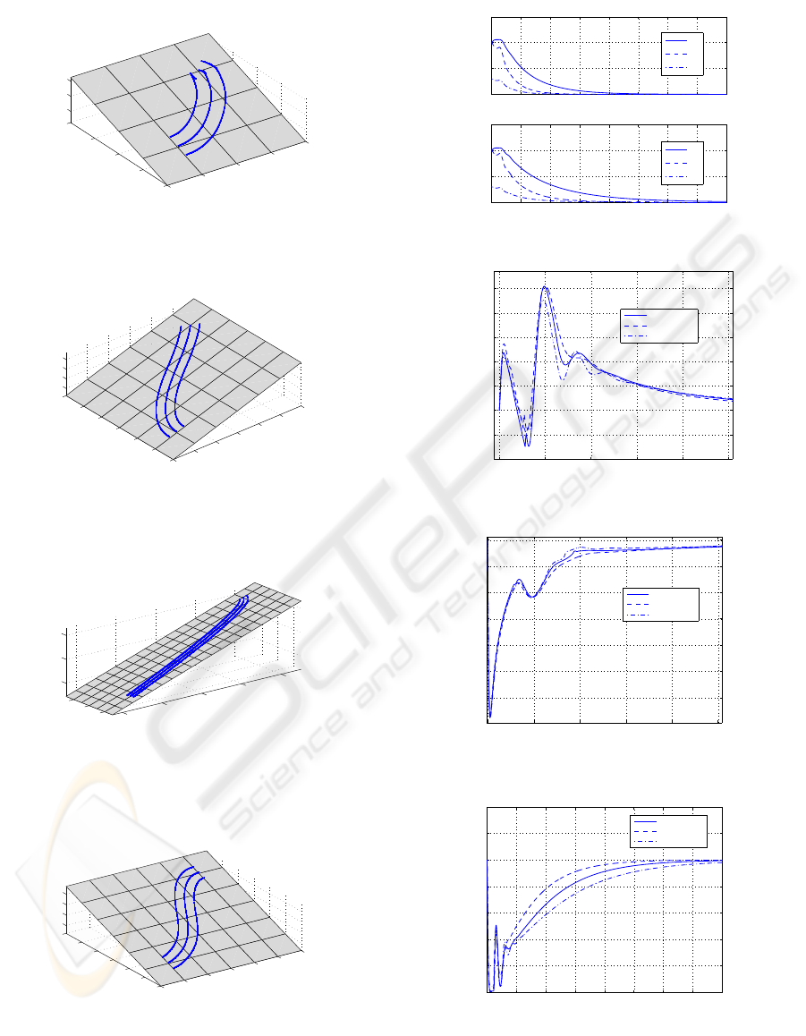
4 SIMULATION RESULTS
In this section we present the simulation results for the
closed-loop system. The inclination of the plane is of
30% for all the simulations. ATOM succeeds to reach
the origin at the desired orientation starting from dis-
tinct initial conditions. Below we display four exam-
ples:
1. coming from up right, Fig. 4(a)
x
c
o
= 1 , y
c
o
= 1 and u
T
3
i = −
√
2/2
2. coming from up left, Fig. 4(b)
x
c
o
= −2 , y
c
o
= 2 and u
T
3
i = −
√
2/2
3. coming from down right, Fig. 4(c)
x
c
o
= 2 , y
c
o
= −7 and u
T
3
i = 0
4. coming from down left, Fig. 4(d)
x
c
o
= 1 , y
c
o
= 1 and u
T
3
i = −
√
2/2
Furthermore, we test the controller performance
versus the parameter uncertainties. We recall here
that the controller is composed of three-imbricated
loops. The inner loop, based on input-output lin-
earization, is obviously dependent of the robot para-
meters. As for the intermediate loop, the judicious
choice of the function ξ
1
allowed a linear dependence
between the heading acceleration of the robot and this
function. Therefore, we were able to implement a lin-
ear controller C(s), with constant parameters. For
the outer loop the choice of the sliding-mode control
and the auxiliary constant input v
0
rendered the con-
troller less dependent of the system parameters. Note
that the choice of the controller parameters was not
a simple task since the system itself is nonsymmet-
ric, due to the up and down motion of ATOM on the
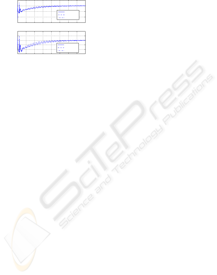
inclined plane. Therefore, we show two simulations
of ATOM moving on the same inclined plane with a
slope of 30%, except that the robot and terrain pa-
rameters seen by the controller are over- and under-
estimated, respectively. The error on the normal vec-
tor to the ground is of 10%, while the error on the
moments of inertia of the rigid bodies composing the
robot and the offset d between the geometric and cen-
ter of mass are of 20%. In both cases, i.e., under- and
over-estimation, ATOM succeeds to reach the origin
with the desired orientation, which can be verified by
looking to the evolution in time of the x−, y−, and
z− components of C
o
depicted in Fig. 4(a). The time
history of the signals v
c
, ω
3p
, and ξ
1
are displayed in
Fig. 4(b), (c), and (d), respectively. The torques ap-
plied to the wheels in Fig.5.
ROBUST POSTURE CONTROL OF A MOBILEWHEELED PENDULUM MOVING ON AN INCLINED PLANE
39
−0.5
0
0.5
1
1.5
−0.5
0
0.5
1
1.5
0
0.2
0.4
x (m)
y (m)
z (m)
(a)
−2.5
−2
−1.5
−1
−0.5
0
0.5
−0.5
0
0.5
1
1.5
2
2.5
0
0.2
0.4
0.6
y (m)
x (m)
z (m)
(b)
0
1
2
−8
−6
−4
−2
0−2
−1
0
y (m)
x (m)
z (m)
(c)
−2.5
−2
−1.5
−1
−0.5
0
0.5
−2.5
−2
−1.5
−1
−0.5
0
0.5
−0.6
−0.4
−0.2
0
x (m)
y (m)
z (m)
(d)
Figure 3: Manoeuvres performed by ATOM on the inclined
plane: reaching the origin at the desired orientation from (a)
up right; (b) up left; (c) down right; and (d) down left.
0 5 10 15 20 25 30 35 40
0
0.5
1
1.5
over estimation
0 5 10 15 20 25 30 35 40
0
0.5
1
1.5
Time (s)
under estimation
x
Co
y
Co
z
Co
x
Co
y
Co
z
Co
(a)
0 2 4 6 8 10
−0.2
−0.1
0
0.1
0.2
0.3
0.4
0.5
Time (s)
v
c
(m/s)
exact param.
over estimat.
under estimat.
(b)
0 2 4 6 8 10
−1.2
−1
−0.8
−0.6
−0.4
−0.2
0
Time (s)
ω
3p
(rd/s)
exact param.
over estimat.
under estimat.
(c)
0 5 10 15 20 25 30 35 40
−1
−0.8
−0.6
−0.4
−0.2
0
0.2
0.4
ξ
1
Time (s)
exact param.
over estimat.
under estimat.
(d)
Figure 4: Controller performance versus parameters uncer-
tainties: time-history of: (a) the x−, y−, and z− compo-
nents of C
o
; (b) v
c
; (c) ω
3p
; and (d) ξ
1
.
ICINCO 2006 - ROBOTICS AND AUTOMATION
40
0 5 10 15 20 25 30 35 40
−3
−2
−1
0
1
τ
1
(N.m)
0 5 10 15 20 25 30 35 40
−1.5
−1
−0.5
0
0.5
1
τ
2
(N.m)
Time (s)
exact param.
over estimat.
under estimat.
exact param.
over estimat.
under estimat.
(a)
Figure 5: Controller performance versus parameters uncer-
tainties: time history of τ
1
and τ
2
.
5 CONCLUSION
The work reported here delivers a robust posture con-
troller for a MWP-class robot moving on an inclined
plane. The challenging issue in this design is to be
able to control the posture of the robot simultaneously
while stabilizing of the central body, which results in
the absence of friction. Unlike previous attempts to
control such systems, our controller is global and less
sensitive to errors in the parameters estimation. We
show that deep insight into the internal dynamics of
the system, in conjunction with proper selection of
a coordinate system and the system output function,
are instrumental in the construction of feedback con-
trollers for nonholonomic systems underlying unsta-
ble zero-dynamics.
Future work will focus on generalization of the mo-
tion of the robot to a warped, smooth surface.
ACKNOWLEDGEMENTS
This work was made possible by NSERC (Canada’s
Natural Sciences and Engineering Research Council)
Grant OGP4532.
REFERENCES
D. L. Kamen, R. R. Ambrogi, R. J. Duggan, R. K. Heinz-
mann, B. R. Key, A. Skoskiewicz, P. K. Kristal, 1999,
“Transportation Vehicles and Methods”, US patent
5,971,091.
F. Grassser, A. D’Arrigo, S. Colombi and A. C. Rufer, 2002,
“JOE: A Mobile, Inverted Pendulum”, IEEE Trans.
Industrial Electronics 49, No. 1, pp. 107-114.
A. Salerno and J. Angeles, 2004, “The Control of Semi-
Autonomous Self-Balancing Two-Wheeled Quasi-
holonomic Mobile Robots”, Proc. 15th CISM-
IFToMM Symposium on Robot Design, Dynamics and
Control (RoManSy), Montreal, June 14-18.
G. Campion, B. d’Andrea-Novel and G. Bastin, 1990,
“Controllability and State Feedback Stabilizability of
Non Holonomic Mechanical Systems”, Advanced Ro-
bot Control, Proc. of the International Workshop on
Nonlinear and Adaptive and Control, Issues in Robot-
ics, Grenoble, November 21-23
C. Samson, K. Ait-Abderrahim, 1999, “Mobile Robot Con-
trol Part 1: Feedback Control of a Nonholonomic
Wheeled Cart in Cartesian Space”, INRIA, Rapport
de Recherche, No.1288, October.
A. Astolfi, 1994, “On the Stabilization of Nonholo-
nomic Systems”, Proc. 33rd Conference on Decision
and Control, Lake Buena Vista, December 14-16,
pp. 3481-3486.
C. Canudas de Wit, O. J. Sordalen, 1992, “Exponential Sta-
bilization of Mobile Robots with Nonholonomic Con-
straints”, IEEE Trans. Automatic Control 37, No. 11,
pp. 1791-1797.
D. Chwa, 2004, “Sliding-Mode Tracking Control of Non-
holonomic Wheeled Mobile Robots in Polar Coordi-
nates”, IEEE Trans. Control Systems Technology 12,
No. 4, pp. 637-644.
J. Guldner, V. I. Utkin, 1994, “Stabilization of Nonholo-
nomic Mobile Robots Using Lyapunov Functions for
Navigation and Sliding Mode Control”, Proc. 33rd
Conference on Decision and Control, Lake Buena
Vista, December 14-16, pp. 2967-2972.
K. Pathak, J. Franch and S. K. Agrawal, 2005, “Velocity
and Position Control of a Wheeled Inverted Pendulum
by Partial Feedback Linearization”, IEEE Trans. Ro-
botics 21, No. 3, pp. 505-513.
D. S. Nasrallah, J. Angeles and H. Michalska, 2005,
“Modeling of an Anti-Tilting Outdoor Mobile Robot”,
ASME Proc. 5th International Conference on Mut-
libody Systems, Nonlinear Dynamics, and Control,
Long Beach, September 25-28.
D. S. Nasrallah, J. Angeles and H. Michalska, 2006, “Veloc-
ity and Orientation Control of an Anti-Tilting Mobile
Robot Moving on an Inclined Plane”, IEEE Proc. In-
ternational Conference on Robotics and Automation,
Orlando, May 15-19, pp. 3717-3723.
S. Sastry, 1999, Nonlinear Systems: Analysis, Stability, and
Control, Springer-Verlag.
R. Marino, 1986, “On the largest feedback linearizable sub-
system”, Systems and Control Letters 6, pp. 345–351.
D.S. Nasrallah, J. Angeles and H. Michaslka, 2006, “The
Largest Feedback-Linearizable Subsystem of a Class
of Wheeled Robots Moving on an Inclined Plane”,
to appear in Proc. 16th CISM-IFToMM Symposium
on Robot Design, Dynamics and Control (RoManSy),
Warsaw, June 20-24.
ROBUST POSTURE CONTROL OF A MOBILEWHEELED PENDULUM MOVING ON AN INCLINED PLANE
41
