NEURAL NETWORK MODEL BASED ON FUZZY ARTMAP FOR

FORECASTING OF HIGHWAY TRAFFIC DATA

D. Boto-Giralda, M. Antón-Rodríguez, F. J. Díaz -Pernas, J. F. Díez Higuera

Departamento de Teoría de la Señal, Comunicaciones e Ingeniería Telemática

ETSIT Universidad de Valladolid, Campus Miguel Delibes s/n, 47011 Valladolid, España

Keywords: Fuzzy ARTMAP, travel cost estimates, ATIS.

Abstract: In this article, a neural network model is presented for forecasting the average speed values at highway

traffic detectors locations using the Fuzzy ARTMAP theory. The performance of the model is measured by

the deviation between the speed values provided by the loop detectors and the predicted speed values.

Different Fuzzy ARTMAP configuration cases are analysed in their training and testing phases. Some ad-

hoc mechanisms added to the basic Fuzzy ARTMAP structure are also described to improve the entire

model performance. The achieved results make this model suitable for being implemented on advanced

traffic management systems (ATMS) and advanced traveller information system (ATIS).

1 INTRODUCTION

Traditional models of traffic congestion and

management lack the adaptability and sophistication

needed to effectively and reliably deal with

increasing traffic volume on certain road stretches.

A realistic estimate of planned routes travel cost

with reasonable accuracy is essential for successful

implementation on an advanced traveller

information system (ATIS) for use in an intelligent

transportation system (ITS). An ATIS consists of a

route guiding system (RGS) that recommend the

most suitable route based on the traveller’s

requirements, using the information gathered from

various sources as loop detectors and probe vehicles.

The success of an RGS will depend on its ability to

predict the anticipatory travel cost in addition to the

historical and real-time travel cost. (Dharia, A. and

Adeli, H., 2003)

Several aspects should be taken into account to

evaluate the travel cost such as distance, time,

economy, danger or personal preferences. From the

distance point of view, the travel cost quantification

will be strictly static, only dependent on the sum of

the stretches length. A time based estimate will be

dynamic and dependent on multiple factors. It could

be directly measured or by the distance-speed

relationship. For a economic estimate, toll fares,

vehicle consumption and wear will be considered.

Road accident risks as well as driving easiness at

some particular stretches might be a decisive factor

to rule out a route. Finally the traveller’s preferences

for route services or particular scenarios such as

mountain or landscape roads could affect the

decision eventually. This article will focus on speed

estimate in road stretches with traffic detectors using

a Fuzzy ARTMAP neural network structure. As said

before, speed may be used to calculated the travel

time cost as long as distance is known.

Neural network computing applied to travel cost

forecast appeared to overcome the shortcomings of

preceding methods whose forecasts deteriorate over

multiple time steps (Park, D. and Rilett, L.R., 1999).

A neural network provides a mapping between a set

of inputs and corresponding outputs (Adeli, H. and

Hung, S.L., 1995). The network is trained to learn

this mapping using a number of training examples.

Backpropagation (BP) is the most widely used

neural network model in civil engineering

applications, primarily due to its simplicity.

However, backpropagation has shortcomings,

including a very slow rate of convergence and

arbitrary and problem-dependent selection of the

learning and momentum ratios (Adeli, H. and Hung,

S.L., 1994).

A neural model for forecasting the freeway link

travel time using counter propagation neural (CPN)

network is presented in (Dharia, A. and Adeli, H.,

2003). There, it was showed that CPN model was

nearly two orders of magnitudes faster than BP

training algorithm for the same level of accuracy. In

Boto-Giralda D., Antón-Rodríguez M., J. Díaz -Pernas F. and F. Díez Higuera J. (2006).

NEURAL NETWORK MODEL BASED ON FUZZY ARTMAP FOR FORECASTING OF HIGHWAY TRAFFIC DATA.

In Proceedings of the Third International Conference on Informatics in Control, Automation and Robotics, pages 19-25

DOI: 10.5220/0001213000190025

 SciTePress

this article, a neural network model based on Fuzzy

ARTMAP is presented for forecasting the average

speed values at highway traffic detectors locations.

Faster as the aforesaid CPN model, the presented

model gives lightly better average errors in

forecasting values in more realistic both training and

testing scenarios.

2 FUZZY ARTMAP BASIS

The Fuzzy ARTMAP, introduced by (Carpenter et

al., 1992) is a supervised network composed of two

Fuzzy ARTs (ART

and ART

) interconnected by a

series of connections between their output layers.

Each connection has an associated weight value (w

)

between 0 and 1, and may be considered as the

membership function value in the fuzzy sets theory

of the corresponding network category.

ART

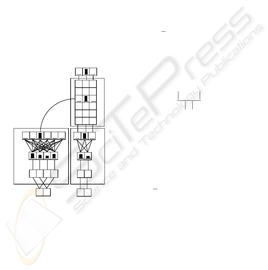
Figure 1: Sample Fuzzy ARTMAP network.

These connections form what is called the map

field F

. The weights of the map field are all

initialised to 1. The map field has two parameters:

the learning rate β

, and vigilance criterion ρ

, and

an output vector x

. Figure 1 shows a graphic

sample representation of a Fuzzy ARTMAP

network.

The input data of both ART

and ART

are

normalized values, between 0 and 1 (minimum and

maximum expected input values respectively), and

form the network input vectors a and b. This

normalization ensures a proportional response of the

network from the input data. Input vector of ART

put in complement coding form, resulting in vector

A. Complement coding is not necessary in ART

the input vector B directly presented to the network.

2.1 Training

Fuzzy ARTMAP networks usage requires a training

process before being able to classify input data. In

this process, a vector representing a data pattern is

presented to ARTa, and a vector which is the desired

output corresponding to this pattern is presented to

ART

. The relationship between these two vectors is

learned through the weight values of the map field.

The vigilance criterion of ART

, ρ

, varies during

learning from a initial value called the baseline

vigilance

. The vigilance parameter of ART

, ρ

is set to 1 to perfectly distinguish the desired output

vectors.

When vectors A and B are presented to ART

and

ART

, both networks soon enter resonance. The map

field vigilance criterion is then evaluated to verify if

the winning neuron of ART

corresponds to the

desired output vector presented to ART

. This

criterion is:

≥

∧

(1)

where y

is the output vector of ART

, J is the index

of the winning neuron on the output layer of ART

corresponds to the weights of the connections to

the Jth neuron of the output layer of ART

and

∈[0,1] is the vigilance criterion of the map field.

If the criterion is not respected, the vigilance of

ART

is increased just enough to select another

winning neuron (ρ

>|A∧w

|/|A| ) and the vector A is

repropagated in ART

When the vigilance criterion is respected, the

vigilance value of ART

is set to its initial baseline

value

and the map field learns the association

between vectors A and B by modifying its weights

as follows:

(

)

Jab

wxw

ββ

−+= 1

(2)

The weights in ART

are also modified as:

(

)( )

JaJaJ

wwAw

−

∧

(3)

In practice, the ART

learning rate, β

, is set equal

to β

, or simply β, defining the learning network

capability.

ICINCO 2006 - INTELLIGENT CONTROL SYSTEMS AND OPTIMIZATION

2.2 Classifying

During the training process the weight values of the

Fuzzy ARTMAP were updating, as new patterns

were presented to the network, till they reached a

final value. At this point the network can be used as

a classifier of the vector data presented to ART

ART

is not used during this classifying process and

learning network capability is deactivated (β=0).

ART

will establish a winning node on its

output layer from each input vector A presented to

the network. The output vector of the map field is

then set to:

wx =

(4)

where J is the index of the winning node on output

layer of ART

, and w

is the corresponding weight

values vector on the map field . The index J of this

component is the number of the category in which

the input vector A has been classified. The use of the

map field is thus to associate a category number to

each neuron of ART

’s output layer. However, not

just the category that best fits an input is the only

result of the classifying process. The weight values

associated with this category may also be useful to

get ulterior information about the relationship

between the input vector and the categories learned

by the network in the training process.

3 WORKING MODEL

3.1 Training the Network

The data for this experiment were collected through

the Freeway Performance Measurement System

(PeMS) project, and could be obtained thanks to the

Next Generation Simulation (NGSIM) and Federal

Highway Administration (FHWA) web page at

http://ngsim.fhwa.dot.gov. PeMS project was

conducted by the Department of Electrical

Engineering and Computer Sciences at the

University of California, at Berkeley, with the

cooperation of California Department of

Transportation. Available data from 5 detector

stations on US 101 South for 11 days, from June 8 to

June 22, excluding the weekends, are provided in

this data set. Speed, volume and occupancy at each

detector for the 5-minute time step are presented at

each detector in each lane.

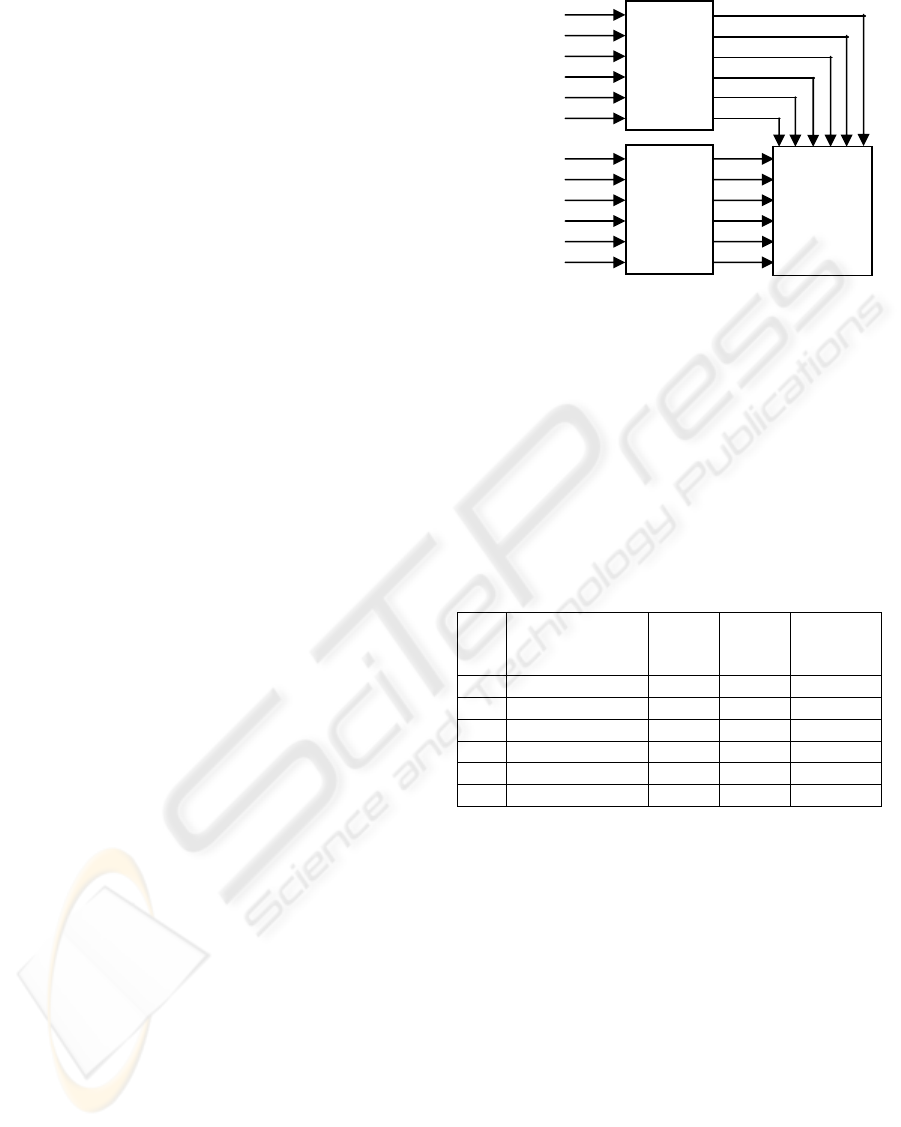
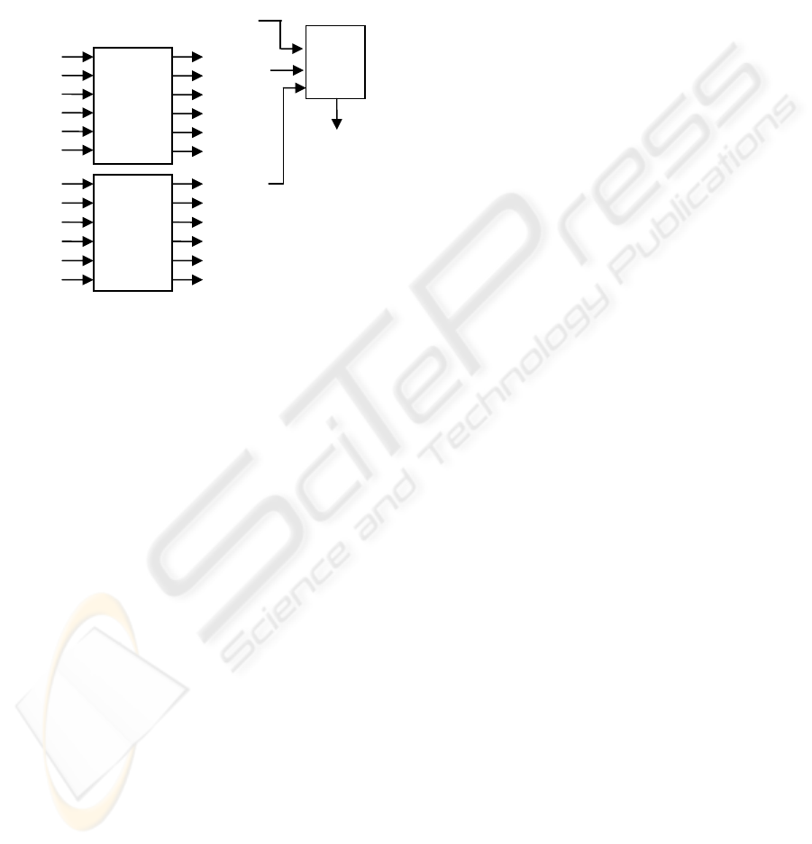
Figure 2: Fuzzy ARTMAP training structure. v

(t):

training speed value at instant t; v

(t): training speed

categorized value at instant t.

Average speed data from June 13 to June 17 (5

consecutive weekdays, making a total of 1440

samples) collected from two stations with different

traffic congestion levels (717486, light; 717489,

heavy), were employed to train the net. Figure 2

shows the structure of the Fuzzy ARTMAP during

this process

Table 1: Training cases.

Case

Input training

subsets time step

(min)

ART

input

nodes

ART

input

nodes

No. of

Categories

A 6*5 6 1 9

B 6*5 6 1 81

C 6*5 6 6 81

D 6*5 4 4 81

E 6*5 8 8 81

F 1*5 6 6 81

Six different structure model cases, shown in

Table 1, were considered with different number of

input and output nodes, categories and time step

between consecutive input training subsets. In Case

A, six ART

input nodes and one ART

input node

were used to associate six consecutive 5-min time

step normalized past speed values to one categorized

future speed value in the map field of the Fuzzy

ARTMAP, F

. This categorized speed value is

calculated as the average of the six 5-min time step

speed values following the normalized speed values

presented to ART

, and categorized into one of 9

possible categories. Numerically, these categories

are linearly spaced and normalized speed values in

the range of 0-80 mph. In Case B, and following

ones, the number of categories were increased to 81.

In Case C, each six consecutive 5-min time step

normalized past speed values presented to ART

)

-5)

-10)

-15)

-20)

(

-25

)

ART

+5)

+10)

+15)

+20)

+25)

(

+30

)

ART

NEURAL NETWORK MODEL BASED ON FUZZY ARTMAP FOR FORECASTING OF HIGHWAY TRAFFIC DATA

were associated to six consecutive 5-min time step

normalized future speed values presented to ART

In Case D and E the number of input nodes were

changed to 4 and 8 respectively. Finally in Case F,

with six input nodes anew, the consecutive sets of

values presented to the ART

and ART

were 5

minutes ahead of the former, instead of 30 minutes.

A one-shot stable learning configuration, as

shown in Table 2, has been adopted: conservative

limit (α≅0) and fast learning (β=1), holding for

fuzzy ART modules with constant vigilance

(Carpenter, G.A. et al., 1992).

Table 2: Training configuration network parameters.

α β

0.001 1 0 0.95 0.001

3.2 Testing the Network

Average speed data from June 20 to June 22 (3

consecutive weekdays following the training ones,

making a total of 864 samples) collected from the

same two stations that in the training process and

shown in

Figure 4.(a) and Figure 5.(a), were employed

to make a test of the speed forecasting net capability.

A test performance was made for each training case.

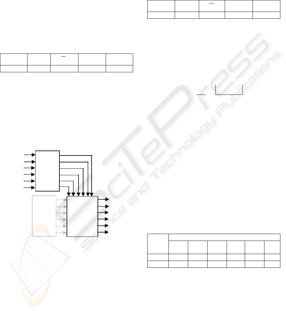
Figure 3: Fuzzy ARTMAP testing structure. vts(t): testing

speed value at instant t; vp(t): forecasting speed value for

instant t.

Figure

3 shows the structure of the Fuzzy ARTMAP

during this process. Sets of consecutive 5-min time

step normalized speed testing values were presented

to ART

. ART

in testing phase is not used. A

number of forecasting speed values, equals to the

number of input nodes in ART

in the training

phase, were obtained from each set. These

forecasting speed values were calculated from the

weight vectors of the map field F

, w

, multiplying

the selected weight vector, w

, by the speed value

associated to the higher training category.

The fuzzy ARTMAP configuration for the testing

phase was similar to the one adopted in the training

phase but with the learning capability deactivated

(β=0), as shown in

Table 3.

Table 3: Testing configuration parameters.

α β

0.001 0 0 0.95 0.001

3.3 Forecasting Results

The Fuzzy ARTMAP model have been implemented

in MATLAB

Release 12 technical language on a

mobile AMD Athlon

™

XP 2000+ computer. In order

to measure the forecasting accuracy, an average

error term was defined in the following form:

()

[] []

[]

∑

−

tvtv

100

(5)

where N is the number of predicted speed values;

[t], the predicted speed value for moment t; v

[t],

the testing speed value measured by the station

detector at moment t.

Figure 4 and Figure 5 show the forecasting speed

(b) and the forecasting error (c) values over the

testing days time. The maximum error values occur

close to high traffic congestion situations in 717489

station, when vehicles speed changes too fast in the

5-min step time. This maximum error values are

dramatically high but are quickly reduced as the next

forecasting speed values are available. Hence, global

error performance keeps a satisfactory level. Table 4

shows the average error in forecasting speed for the

considered cases.

Table 4: Average error in forecasting speed.

E(%)

Station

Case

717486 4.12 2.91 3.16 3.77 3.12 2.64

717489 14.78 13.95 10.96 9.67 15.84 7.78

)

-5)

-10)

-15)

-20)

-25)

ART

+5)

+10)

+15)

+20)

+25)

(

+30

)

ICINCO 2006 - INTELLIGENT CONTROL SYSTEMS AND OPTIMIZATION

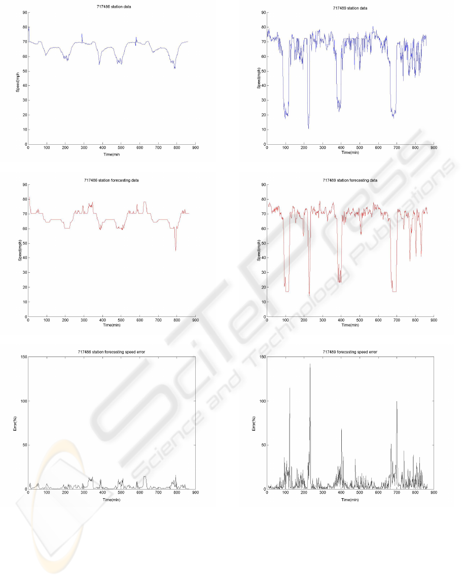
(a) 717486 station detector speed data

(b) 717486 station forecasting speed data

Figure 4: 717486 station data and forecasting results.

Case B improves Case A forecasting precision by

simply increasing the number of categories,

particularly with the 717486 station in which all

speed values concentrate in a range of 30 mph.

Forecasting precision for 717489 station, in

which speed values change quickly close to high

congestion situations, strongly improves in Case C

as more predicted speed values are given (six instead

(a) 717489 station detector speed data

(b) 717489 station forecasting speed data

Figure 5: 717489 station data and forecasting results.

of one) for the 30-min forecasting time interval

considered. Applying no interpolation rule, six is the

highest number of predicted values since detectors

present new data each 5 minutes.

The increase in the number of nodes in Case E

implies that both the time interval of past speed

values presented to the net and the time interval of

forecasting speed values are longer, since the

NEURAL NETWORK MODEL BASED ON FUZZY ARTMAP FOR FORECASTING OF HIGHWAY TRAFFIC DATA

number of nodes in ART

and ART

were equal in

the training process. For the 717489 station, with

speed values changing quickly close to high traffic

congestion situations, the longer the forecasting time

interval , the bigger the error will be. In Case D, the

opposite situation occurs but the processing time

increases substantially for the same forecasting time

interval. No significantly error variation for 717486

station in Cases D and E.

Figure 6: Case F model structure.v

(t): testing speed value

at instant t; v

(t): ith forecasting speed value for instant t;

(t): forecasting speed value for instant t.

The best error performance is achieved in Case F

in which several forecasting speed values (up to the

number of input nodes) are obtained for a particular

moment into the future (due to the time overlap of

the input set speed values). An average of them is

then made to get the final forecasting speed value.

Figure 6shows the model structure designed for this

particular case.

3.4 Comparative Results

The average errors in forecasting values presented in

(Dharia, A. and Adeli, H., 2003) for BP and CPN

models with the same duration of time step (5min)

and the same number of input and output nodes (6),

were slightly higher (11.5% and 10.9% respectively)

than the one achieved for the Case F (7.8% for the

station with the most congested traffic level) in the

Fuzzy ARTMAP model. However, speed travel

values, instead of travel time values, were predicted

in the model presented in this article and real traffic

data were used instead of simulated traffic data.

Case F did not take more than 10 seconds (a rough

measure was made) of processing time to carry out

both training and testing phases with the conditions

described above. BP and CPN models took 312.7

and 3.8 seconds respectively just for the training

process. Convergence behaviour of Fuzzy ARTMAP

networks are faster and more independent of the

initial weights than Back or Counter propagation

networks. Actually, training convergence can be

guaranteed as far as Fuzzy ART Stable Category

Learning Theorem (Carpenter, G.A. et al., 1992) is

satisfied.

4 CONCLUSIONS

The Fuzzy ARTMAP neural network model

described in this article provides an appropriated

forecasting travel cost mechanism, in terms of

average speed values for being integrated in travel

cost estimates systems supplied with traffic dynamic

parameters such as speed, occupancy or volume

data. Multiple training and working configurations

for the network are possible in order to match host

system requirements, all of them with a remarkable

time processing and forecasting error performance.

Forecasting test results obtained accuracy levels

under the 8% of precision from real congested

highway traffic data. A figure slightly lower than

previous neural network models developed for

highway traffic predictions. So it represents a

promising challenge in the evolution of neural

networks appliance to intelligent transportation

system (ITS).

ACKNOLEDGEMENTS

NGSIM Website - Home of the Next Generation

Simulation Community, at http://ngsim.camsys.com

- for the traffic data set.

REFERENCES

Adeli, H., 2002. “Automatic detection of traffic incidents

using data obtained from sensors embedded in

intelligent freeways ”. Sensor Review; Volume: 22

Issue: 2; 2002 Research paper.

Adeli, H., Hung, S.L., 1995. “Machine Learning-Neural

Networks, Genetic Algorithms, and Fuzzy Systems”.

Wiley, New York.

Adeli, H., Hung, S.L., 1994. “An adaptive conjugate

gradient learning algorithm for efﬁcient training of

neural networks”. Applied Mathematics and

Computatio n 62 (1), 81–100.

Carpenter, G.A., 2003. “Default ARTMAP”. Neural

Networks, 2003. Proceedings of the International Joint

...

-5)

-10)

-15)

-20)

-25)

-30)

ART

+5)

+10)

+15)

+20)

+25)

+30)

)

-5)

-10)

-15)

-20)

(

-25

)

+5)

+10)

+15)

+20)

+25)

average

module

+5)

ICINCO 2006 - INTELLIGENT CONTROL SYSTEMS AND OPTIMIZATION

Conference on Volume 2, 20-24 July 2003

Page(s):1396 – 1401 vol.2.

Carpenter, G.A., et al., 1992.”Fuzzy ARTMAP: A neural

network architecture for incremental supervised

learning of analog multidimensional maps”. Neural

Networks, IEEE Transactions on Volume 3, Issue 5,

Sept. 1992 Page(s):698 – 713.

Dharia, A. and Adeli, H., 2003. “Neural network model

for rapid forecasting of freeway link travel time”.

Engineering Applications of Artificial Intelligence,

Volume 16, Issues 7-8, October-December 2003,

Pages 607-613.

Jiang, G., et al., 2003. “The study on the application of

fuzzy clustering analysis in the dynamic identification

of road traffic state”. Intelligent Transportation

Systems, 2003. Proceedings. 2003 IEEE. Volume 1,

2003 Page(s):408 – 411 vol.1.

Park, D., Rilett, L.R., 1999. “Forecasting freeway link

travel times with a multilayer feedforward neural

network”. Computer-Aided Civil and Infrastructure

Engineering 14 (5), 357–367.

Wang, X-H, Xiao, J.M.,2003.”A radial basis function

neural network approach to traffic flow forecasting”.

Intelligent Transportation Systems, 2003. Proceedings.

2003 IEEE. Volume 1, 2003 Page(s):614 – 617 vol.1.

NEURAL NETWORK MODEL BASED ON FUZZY ARTMAP FOR FORECASTING OF HIGHWAY TRAFFIC DATA