
IMPROVING TRACKING TRAJECTORIES WITH MOTION
ESTIMATION
J. Pomares, G. J. García, F. Torres
Physics, Systems Engineering and Signal Theory Department. University of Alicante, Alicante, Spain
Keywords: Motion estimation, tracking trajectories, visual control.
Abstract: Up to now, different methods have been proposed to track trajectories using visual servoing systems.
However, when these approaches are employed to track trajectories specified with respect to moving
objects, different considerations must be included in the visual servoing formulation to progressively
decrease the tracking error. This paper shows the main properties of a non-time dependent visual servoing
system to track image trajectories. The control action obtained integrates the motion estimation of the object
from which the features are extracted. The proposed motion estimator employs information from the
measures of the extracted features and from the variation of the camera locations. These variations are
obtained determining the Homography matrix between consecutive camera frames.
1 INTRODUCTION
Now, visual servoing systems are a well-known
approach to guide a robot using image information.
Tipically, visual servoing systems are position-based
and image-based classified (Hutchinson et al. 1996).
Position-based visual servoing requires the
computation of a 3-D Cartesian error for which a
perfect CAD-model of the object and a calibrated
camera are necessary. These types of systems are
very sensitive to modeling errors and noise
perturbations. In image-based visual servoing the
error is directly measured in the image. This
approach ensures the robustness with respect to
modeling errors, but generally an inadequate
movement of the camera in the 3-D Cartesian space
is obtained. On the other hand, it is well known that
image-based visual servoing is locally stable. This
nice property ensures a correct convergence if the
desired configuration is sufficiently near to the
current one. This paper shows the properties of an
approach which employs image-based visual
servoing to track trajectories. This method is not the
main objective of the paper and a more extensive
study of the approach can be seen in our previous
works (Pomares and Torres, 2005).
Once this strategy is defined, the paper focuses on
the extension of the previous mentioned algorithms
to be able to carry out the tracking of image
trajectories when the visual features are in motion.
Previous works, such as (Hutchinson et al. 1996)
have shown the necessity of estimating object
motion and to include this estimation in the control
action in order to decrease the tracking errors. The
motion estimation can be solved using different
algorithms like the one shown in (Pressigout and
Marchand, 2004) based in virtual visual servoing. In
(Bensalah and Chaumette, 1995) an estimator which
employs measurements about the camera velocity is
proposed. However, this method introduces errors in
the estimation due to the non accuracy measurement
of the camera motion. The previous mentioned
algorithms are used to achieve a given configuration
of the features in the image. In this paper, we define
method to improve the estimation of the camera
velocity based on visual information. This method is
used to define a motion estimator to be applied
during the tracking of trajectories.
This paper is organized as follows: The main
aspects of the visual servoing system to track
trajectories are first described in Section 2. Section 3
shows a method to estimate the motion of the object
from which the features are extracted. Section 4,
simulation and experimental results confirm the
validity of the proposed algorithms. The final
section presents the main conclusions arrived at.
97
Pomares J., J. García G. and Torres F. (2006).
IMPROVING TRACKING TRAJECTORIES WITH MOTION ESTIMATION.
In Proceedings of the Third International Conference on Informatics in Control, Automation and Robotics, pages 97-103
DOI: 10.5220/0001212400970103
Copyright
c
SciTePress
2 TRACKING IMAGE
TRAJECTORIES
First, the notation employed and the desired
trajectory to be tracked are described. In this paper,
we suppose that the robot must track a desired
trajectory in the 3D space, γ(t), using an eye-in-hand
camera system. By sampling the desired trajectory,
γ(t), a sequence of N discrete values is obtained,
each of which represents N intermediate positions of
the camera
k
k 1...N∈γ/
. From this sequence, the
discrete trajectory of the object in the image
{
}
k
Sk1...N=∈s/
can be obtained, where
k
s is the
set of M points or features observed by the camera at
instant k,
{}
kk
i
i 1...M=∈s/f
. In the next section, a
non time-dependent visual controller to track the
previous mentioned image trajectory is described.
2.1 Visual Servo Control
The control action obtained from the visual
controller is:
C+
Vff
ˆ
λ=− ⋅ ⋅Jve
(1)
where
C
V
v is the velocity obtained with respect to the
camera coordinate frame;
λ 0> is the gain of the
controller;
+
f
ˆ
J
is the pseudoinverse of the estimated
interaction matrix (Hutchinson et al. 1996);
fd
= ss-e ; s=[f
1
, f
2
,…, f
M
]
T
are the set of features
extracted from the image; s
d
=[f
1
+m
1
Φ
1
(f
1
),
f
2
+m
2
Φ
2
(f
2
),…, f
M
+m
M
Φ
M
(f
M
)]
T
; Φ
i
is the movement
flow for the feature i, m={m
1
, m
2
,…, m
M
}
determines the progression speed.
Now, for the sake of clarity, the sub-index that
indicates which feature is being considered and the
super-index that indicates the instant in which these
features are obtained are omitted. The movement
flow, Φ, is a set of vectors converging towards the
desired trajectory in the image.
We consider, for a given feature, a desired
parameterized trajectory in the image f
d
:Γ → ℑ
where Γ ⊂ ℜ. The coordinates of this trajectory in
the image are f
d
(τ)=[f
xd
(τ), f
yd
(τ)] and f are the
current coordinates of the feature in the image. The
error vector E(f)=(E
x
, E
y
) where E
x
=(f
x
-f
xd
) and
E
y
=(f
y
-f
yd
) is defined, where f
d
=(f
xd
, f
yd
) are the
coordinates of the nearest point to f in the desired
trajectory. The movement flow, Φ, is defined as:
()
(
)
()
()
xd
x
12
yd
y
τ
τ
τ
τ
∂
⎛⎞
⎛∂ ⎞
⎜⎟
⎜⎟
∂
∂
⎜⎟
⎜⎟
Φ= ⋅ − ⋅
⎜⎟
∂
⎜⎟
∂
⎜⎟
⎜⎟
∂
∂
⎝⎠
⎝⎠
U
U
f
E
GG
f
E
ff
(2)
where U is the potential function defined in Section
3.2 and G
1
, G
2
: ℑ → ℜ
+
are weight functions so that
G
1
+ G
2
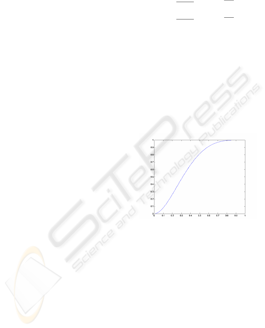
= 1. As can be seen in Equation (2), the
first component of the movement flow mimics the
behaviour of the desired trajectory, and, therefore,
G
1
controls the progression speed of the trajectory in
the image. The purpose of the second term is to
reduce the tracking error, and therefore G
2
controls
the strength of the gradient field. Specifically, to
determine the values of these weight functions we
have used the function shown in Figure 1 and we
have defined the parameter
δ
being a variable that
represents an error value such that if
(
)
1
0
δ
⎛⎞
⎜⎟
⎝⎠
>→ =U GEf (maximum tracking error
permitted).
Figure 1: Evolution of G
2
.
2.2 Potential Function
The potential function U employed in the definition
of the movement flow must attain its minimum
when the error is zero and must increase as f
deviates more from the desired location f
d
. The
visual features are under the influence of an artificial
potential field (U) defined as an attractive potential
pulling the features towards the desired image
trajectory.
I is the image that would be obtained
after the trajectory f
d
(τ) has been represented. The
first step in determining the potential function is to
calculate the gradient I
g
of I. Once the image I
g
has
been obtained, the next step to determine the
potential function is to generate a distance map
(Lotufo and Zampirolli, 2001). The distance map
Weight
G
2
U(E)/δ
ICINCO 2006 - ROBOTICS AND AUTOMATION
98
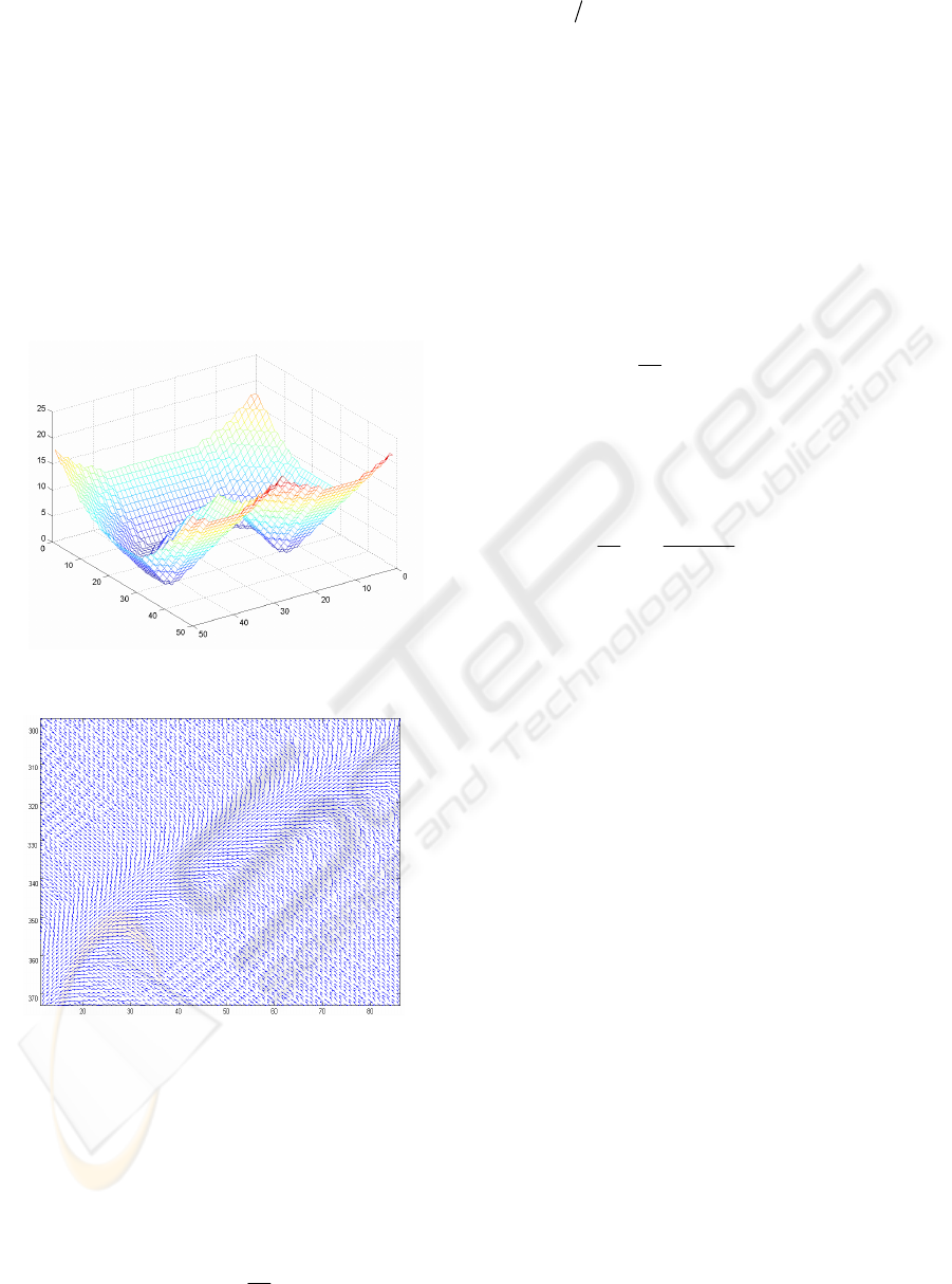
creates a distance image I
d
of the image I
g
, so that
the value of I
d
at the pixel x is the Euclidean distance
from x to the complement of I
g
. In Figure 2, a three-
dimensional representation of the distance map is
shown for a given feature. In this figure the value of
z coordinate represents the distance between each
pixel and the nearest pixel to it in the desired
trajectory. This representation shows the distribution
of the potential function, U. Using this potential
function and following the steps described, the
movement flow can be obtained. In Figure 3 a detail
of the movement flow obtained for the trajectory
whose distance map is represented in
Figure 2, is
shown.
Figure 2: Distance map.
Figure 3: Movement flow.
3 TRACKING MOVING OBJECTS
In order to track trajectories specified with respect to
moving objects, the motion of the object must be
included in the control action proposed in (1). Doing
so, the new control action will be:
C+
ff
ˆ
ˆ
λ
∂
=− ⋅ ⋅ −
∂
J
t
e
ve
(3)
where
ˆ
∂
∂te represents the estimation of the
variations of
+
ff
ˆ
=
⋅Jee
due to the movement of the
object from which the features are extracted. As is
shown in (Bensalah and Chaumette, 1995), the
estimation of the velocity of a moving object tracked
with an eye-in-hand camera system can be obtained
from the measurements of the camera velocity and
from the error function. Thus, from Equation (1) the
value of the estimation of the error variation due to
the movement of the tracked object can be obtained
in this way (to obtain an exponential decrease of the
error it must fulfil that
λ
=
−⋅
ee):
C
ˆ
∂
=
−
∂
t
e
ev
(4)
From Equation (4), the value of the motion
estimation can be obtained using the following
expression:
C
kk1
k1
k
ˆ
−
−
−
∂
⎛⎞
=−
⎜⎟
∂Δ
⎝⎠
tt
ee
e
v
(5)
Where
Δ
t can be obtained determining the delay at
each iteration of the algorithm, e
k
and e
k-1
are the
error values at the instants k and k-1, and
C
k1−
v is the
camera velocity measurement at the instant k-1 with
respect the camera coordinate frame. As is shown in
our previous works (Pomares et al. 2002) the
estimations obtained from Equation (5) depends on
the measurement of the camera motion which cannot
be measured without errors. Therefore, in order to
improve the global behaviour of the system it is
necessary to obtain a more accuracy estimation of
the camera motion.
To compute the camera velocity in the previous
iteration
C
k1
−
v
it is necessary to obtain the rotation
R
k-1
and translation t
dk-1
between the two last frames.
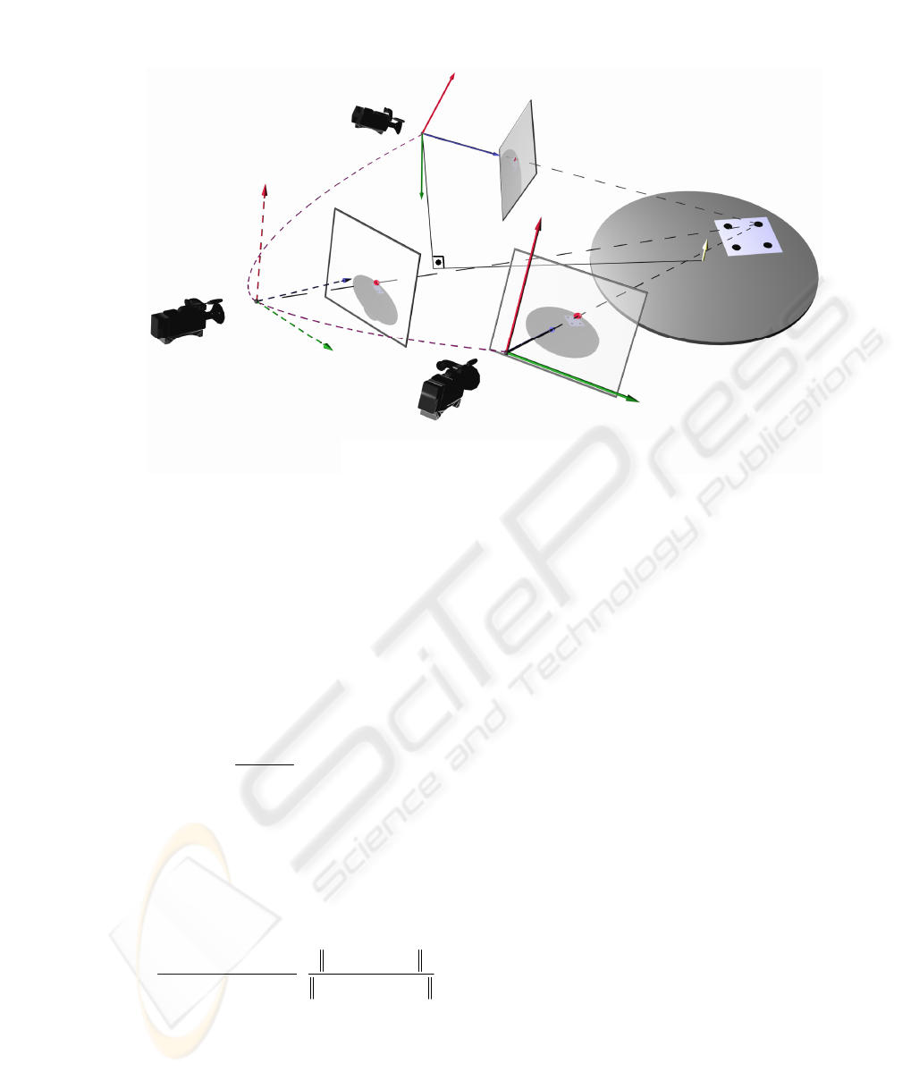
To do so, first of all, we call Π the plane containing
the object. Considering
P a 3D point observed by the
camera, the same point in the image space is
p. With
p
k-1
we represent the position of the feature in the
image captured at instant k-1. In the next image
(which corresponds with the image obtained by the
camera after one iteration of the control loop), the
same point will be located at
p
k
position (see Figure
4). The projective homography
G is defined as:
x axis (pix)
z axis
(pix)
y axis (pix)
IMPROVING TRACKING TRAJECTORIES WITH MOTION ESTIMATION
99
k-1 k-1 k
μβ
=+Gpp
ζ
(6)
where
k-1
μ
is a scale factor,
k-1 dk-1
= AR t
ζ
is the
projection in the image captured by the camera at
time k-1 of the optical centre when the camera is in
the next position, and
β is a constant scale factor
which depends on the distance Z
k
from the contact
surface
to the origin of the camera placed at the
current position:
k
(, )
Z
β
Π
=
dP
(7)
where
(, )ΠdP is the distance from the contact
surface plane to the 3D point. Although
β is
unknown, applying (6) between the instant k-1 (at
previous iteration) and the current camera positions
we can obtain that:
()
()
k-1k-1 k-1k
k-1 k k-1
1
k-1 dk-1 k-1 dk-1 k-1
1
μ
β
⎛⎞
−
∧
=
⎜⎟
⎜⎟
∧
⎝⎠
G
G
AR AR
pp
pp
sign
ptt
(8)
where subscript 1 indicates the first element of the
vector and
A is a non singular matrix containing the
camera internal parameters:
()
()
uu 0
v0
ffcotθ
0f/sinθ
001
⋅−⋅⋅
⎡
⎤
⎢
⎥
=⋅
⎢
⎥
⎢
⎥
⎣
⎦
A
pp u
pv
(9)
where
u
0
and v
0
are the pixel coordinates of the
principal point, f is the focal length,
p
u
and p
v
are the
magnifications in the
u and v directions respectively,
and
θ is the angle between these axes.
If
P is on the plane Π, β is null. Therefore, from (6):
k-1 k-1 k
μ
=
Gpp
(10)
Projective homography
G can be obtained through
expression (10) if at least four points on the surface
Π are given (Hartley and Zisserman, 2000). This
way, we can compute projective homography
relating previous and current positions
G
k-1
. In order
to obtain
R
k-1
and t
dk-1
we must introduce the concept
of the Euclidean homography matrix
H.
From projective homography
G it can be obtained
the Euclidean homography
H as follows:
1−
=HAGA
(11)
From
H it is possible to determine the camera
motion applying the algorithm shown in (Zhang and,
Hanson 1996). So, applying this algorithm between
previous and current positions we can compute
R
k-1
and t
dk-1
.
As iteration time Δt is known, it is now easy to
compute the velocity of the camera at previous
F
k
-2
F
k
F
k
-1
n
P
Z
k
П
p
k
-1
p
k
p
k
-2
R
k
-1,
t
d
k
-1
R
k
-2,
t
d
k
-2
Figure 4: Scheme of the motion estimation.
ICINCO 2006 - ROBOTICS AND AUTOMATION
100
iteration v
k-1
through R
k-1
and t
dk-1
. The linear
component of the velocity is computed directly from
t
dk-1
, whereas the computation of angular velocity
requires taking other previous steps. The angular
velocity can be expressed as:
k -1 k -1 k -1 k -1
()= T
ωϕϕ
(12)
where
[
]
k-1 k-1 k-1 k-1
α
βγ
=
ϕ
are the Euler angles
ZYZ obtained from
R
k-1
,
k-1
ϕ
are the time derivative
of the previous Euler angles and:
k-1 k-1 k-1
k-1 k-1 k-1 k-1 k-1
k-1
0 sin cos sin
()0cos sin sin
10 cos
ααβ
ααβ
β
−
⎛⎞
⎜⎟
=
⎜⎟
⎜⎟
⎝⎠
T
ϕ
(13)
Applying (7) it is possible to compute the angular
velocity of the camera to achieve current position
from the previous iteration. This way linear and
angular velocity of the camera between the two
iterations are computed:
dk-1
tk-1
k-1
k-1
k-1 k-1 k-1
()
⎛⎞
⎛⎞
⎜⎟
==
Δ
⎜⎟
⎜⎟
⎜⎟
⎝⎠
⎝⎠
T
t
t
v
v
ω
ϕϕ
(14)
4 RESULTS
4.1 Experimental Setup
The system architecture is composed of an eye-in-
hand PHOTONFOCUS MV-D752-160-CL-8
camera at the end-effector of a 7 d.o.f. Mitsubishi
PA-10 robot. The camera is able to acquire and to
process up to 100 frames/second using an image
resolution of 320x240. In this paper we are not
interested in image processing issues; therefore, the
image trajectory is generated using four grey marks
whose centres of gravity will be the extracted
features.
4.2 Simulation Results
In this section simulation results are obtained from
the application of the proposed visual servoing
system to track trajectories specified with respect to
moving objects. To do so, the motion estimator
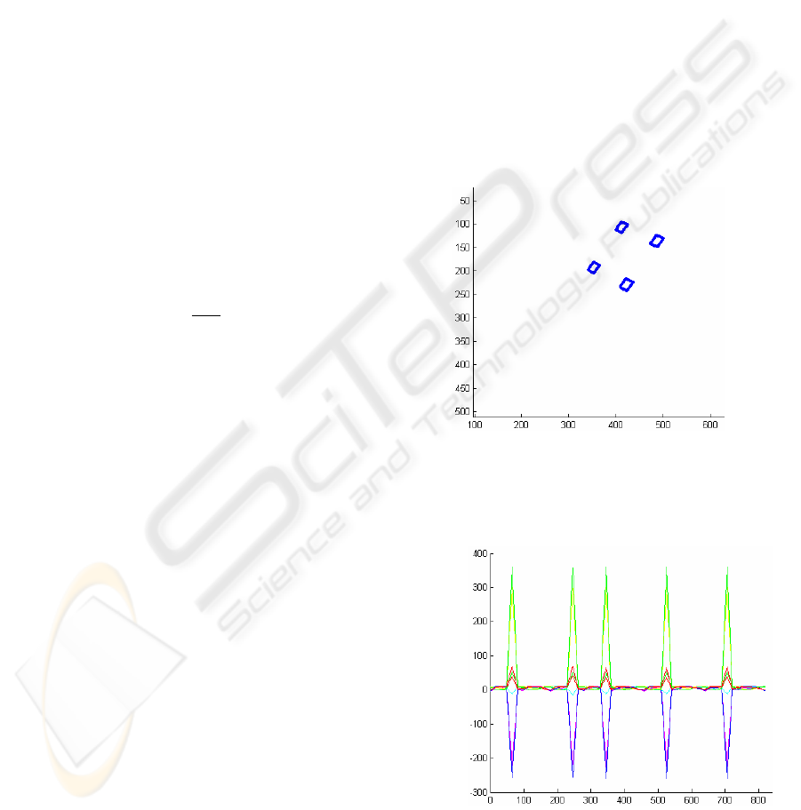
described in Section 3 is used. The motion of the
features extracted during the experiment is shown in
Figure
5. In this figure the evolution of the visual
features observed from the initial camera position is
represented (in this figure we consider that any
control action is applied to the robot). We can see
that the target object describes a periodical and
rectangular motion. To better show the object
motion, in Figure 6 the image error evolution is
represented. As previously, in Figure 6 any control
action is applied to the robot (in this figure the
desired features are the ones provided by the
movement flow). This motion will not end until the
trajectory is completely tracked. Figure 7 shows the
desired image trajectory and the ones obtained
considering and without considering motion
estimation. This figure shows that, using motion
estimation, the system tracks the desired trajectory
avoiding error due to the motion of the object from
which the features are extracted.
Figure 5: Image trajectory observed from the initial
camera position.
Figure 6: Image error due to the object motion.
e
f
(pix.)
Iterations
y
(pix.)
x (pix..)
IMPROVING TRACKING TRAJECTORIES WITH MOTION ESTIMATION
101
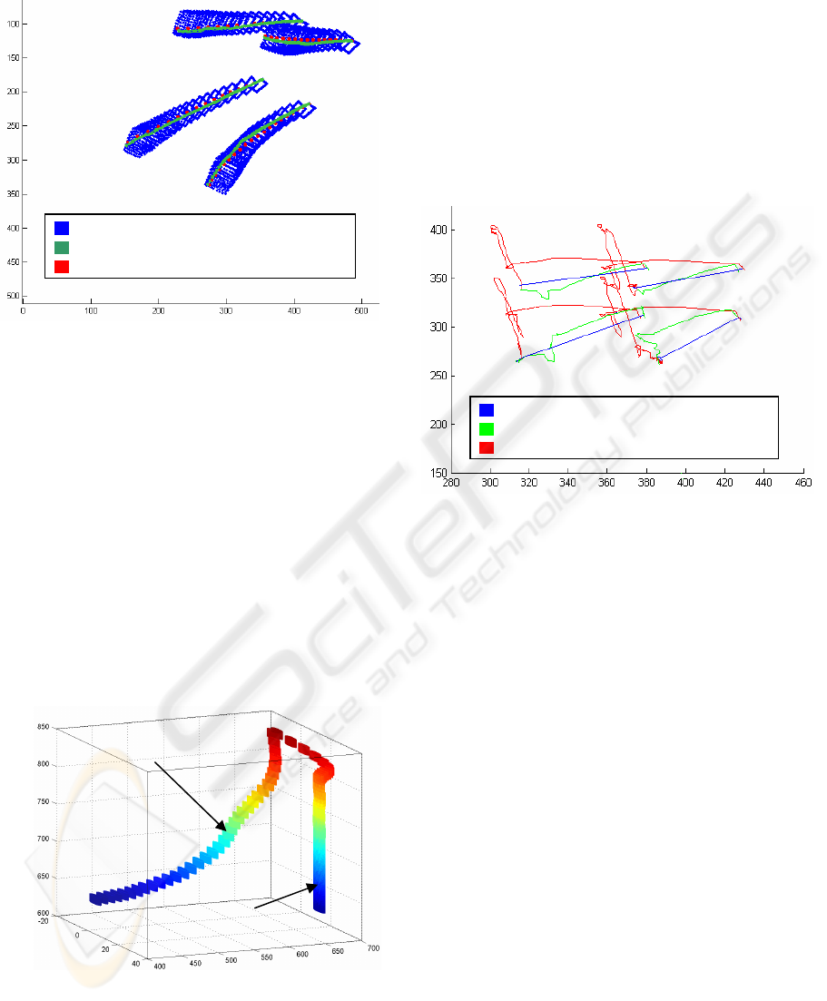
Figure 7: Desired image trajectory and the ones obtained
with and without motion estimation.
4.3 Experimental Results
In order to verify the correct behaviour of the system
the experimental setup described in Section 4.1 is
applied to track trajectories using the proposed
visual servoing system. In Figure 8 the desired
trajectory (without considering motion of the object
from which the trajectory is specified) is shown. In
the same figure is also represented the obtained
trajectory when the object from which the features
are extracted is in motion. We can observe that the
motion is lineal (is not equal to the one described in
section 4.2).
Figure 8: Comparison between the desired 3D trajectory
and the one obtained using motion estimation.
In order to observe the improvement introduced by
the motion estimation in the visual servoing system,
in
Figure 9 a comparison in the image space between
the desired trajectory and the ones obtained with and
without motion estimation is represented. We can
see that using motion estimation the system reduces
rapidly the tracking error due to the motion of the
object. The object motion is not constant, therefore,
when the motion estimation is not carried out, the
error increases quickly when the object velocity
increases. This tracking error is clearly reduced
using the motion estimation proposed in this paper.
Figure 9: Desired image trajectory and the ones obtained
with and without motion estimation.
5 CONCLUSIONS
In this paper we have shown a visual servoing
system to track image trajectories specified with
respect to moving objects. In order to avoid the
errors introduced by the motion, it is required to
include in the control action of the visual servoing
system the effect of this motion. The paper describes
the necessity to obtain a good estimation of the
camera motion and, to do so, a method based on
visual information has been proposed. Simulation
and experimental results show that using the
proposed estimator a good tracking is obtained
avoiding the errors introduced by the motion.
ACKNOWLEDGEMENTS
This work was funded by the Spanish MCYT project
DPI2005-06222 “Diseño, implementación y
experimentación de escenarios de manipulación
inteligentes para aplicaciones de ensamblado y
desensamblado automático” and by the project
Trajectory without motion estimation
Trajectory with motion estimation
Desired Tra
j
ector
y
Desired trajectory
Trajectory with motion estimation
Tra
j
ector
y
without motion estimation
Real trajectory
(with motion)
Desired trajectory
(without motion)
x (mm.) y (mm.)
z
(mm.)
y
(pix.)
x (pix.)
ICINCO 2006 - ROBOTICS AND AUTOMATION
102

GV05/007: “Diseño y experimentación de
estrategias de control visual-fuerza para sistemas
flexibles de manipulación”.
REFERENCES
Bensalah, F., Chaumette, F. 1995. Compensation of abrupt
motion changes in target tracking by visual servoing.
In IEEE/RSJ Int. Conf. on Intelligent Robots and
Systems, IROS'95, Pittsburgh, Vol. 1, pp. 181-187.
Hartley R., Zisserman A. 2000. Multiple view Geometry in
Computer Vision. Cambridge Univ. Press, pp. 91- 92.
Hutchinson, S., Hager, G., Corke, P., 1996. A Tutorial on
Visual Servo Control. IEEE Trans. on Robotics and
Automation, vol. 12, no. 5, pp. 651-670.
Lotufo, R. and Zampirolli, F. 2001. Fast multidimensional
parallel euclidean distance transform based on
mathematical morphology. In Proc. of SIBGRAPI
2001, pp. 100-105.
Pomares, J., Torres, F., Gil, P. 2002. 2-D Visual servoing
with integration of multiple predictions of movement
based on Kalman filter. In Proc. of IFAC 2002 15
th
World Congress, Barcelona, Vol L.
Pomares, J., Torres, F., 2005. Movement-flow based
visual servoing and force control fusion for
manipulation tasks in unstructured environments.
IEEE Transactions on Systems, Man, and
Cybernetics—Part C. Vol. 35, No. 1. Pp. 4 – 15.
Pressigout, M., Marchand, E. 2004. Model-free augmented
reality by virtual visual servoing. In IAPR Int. Conf.
on Pattern Recognition, ICPR'04, Cambridge.
Zhang, Z., Hanson, A.R. 1996. Three-dimensional
reconstruction under varying constraints on camera
geometry for robotic navigation scenarios, Ph.D.
Dissertation.
IMPROVING TRACKING TRAJECTORIES WITH MOTION ESTIMATION
103
