PATTERN TRACKING AND VISUAL SERVOING FOR INDOOR

MOBILE ROBOT ENVIRONMENT MAPPING

AND AUTONOMOUS NAVIGATION

O. Ait Aider, G. Blanc, Y. Mezouar and P. Martinet

LASMEA

UBP Clermont II, CNRS - UMR6602

24 Avenue des Landais, 63177 Aubiere, France

Keywords:

Mobile robot, autonomous navigation, pattern tracking, visual servoing.

Abstract:

The paper describes a complete framework for autonomous environment mapping, localization and navigation

using exclusively monocular vision. The environment map is a mosaic of 2D patterns detected on the ceiling

plane and used as natural landmarks. The robot is able to localize itself and to reproduce learned trajectories

deﬁned by a set of key images representing the visual memory. A speciﬁc multiple 2D pattern tracker was

developed for the application. It is based on particle ﬁltering and uses both image contours and gray scale level

variations to track efﬁciently 2D patterns even on cluttered ceiling appearance. When running autonomously,

the robot is controlled by a visual servoing law adapted to its nonholonomic constraint. Based on the regu-

lation of successive homographies, this control law guides the robot along the reference visual route without

explicitly planning any trajectory. Real experiment results illustrate the validity of the presented framework.

1 INTRODUCTION

For an indoor mobile robot system, the ability to au-

tonomously map its environment and localize itself

relatively to this map is a highly desired property. Us-

ing natural rather than artiﬁcial landmarks is another

important requirement. Several works using monocu-

lar vision for mapping and self localization exist. The

most important difﬁculty is to achieve the generation

of a sufﬁcient number of landmarks which can be ro-

bustly recognized during navigation session with a

near real time rate. Interest points (Se et al., 2001),

straight lines (Talluri and Aggarwal, 1996) and rec-

tangular patterns (Hayet, 2003) were used. The ﬁrst

approaches focused on producing efﬁcient algorithms

to match a set of observed patterns with a subset of the

map primitives (Talluri and Aggarwal, 1996). Multi-

ple sensor data fusion (odometry) was generally used

to achieve real time computing by eliminating ambi-

guities. More recently, the success of real-time track-

ing algorithms simpliﬁed the matching process and

allowed to use structure from motion technics to com-

pute the 3D coordinates of the observed features (Se

et al., 2001).

In this paper, we show how pattern tracking and vi-

sual servoing is used to provide a complete framework

for autonomous indoor mobile robot application. The

focus is done on three main points: i) environment

mapping with autonomous localization thanks to pat-

tern tracking, ii) path learning using visual memory,

iii) path reproducing using visual servoing.

The environment map is a mosaic of 2D patterns

detected on the ceiling plane and used as natural land-

marks. This makes the environment representation

minimalist and easy to update (only vector represen-

tations of the pattern are stored rather than entire im-

ages). During a learning session, landmarks are au-

tomatically detected, added to the map and tracked

in the image. The consistency of the reconstruction is

guaranteed thanks to the pattern tracker which enables

robot pose updating.

A speciﬁc pattern tracker was developed for the ap-

plication. This was motivated by the fact that for re-

alistic robotics applications there is a need for algo-

rithms enabling not only pattern tracking but also au-

tomatic generation and recognition. Among the large

variety of existing tracking methods, model-based ap-

proaches provide robust results. These methods can

use 3D models or 2D templates such as appearance

models (Jurie and Dhome, 2001; Black and Jepson,

1996) or Geometric primitives as contour curves and

CAD description (Marchand et al., 1999; Lowe, 1992;

Pece and Worrall, 2002). Object recognition algo-

rithms based on segmented contours (straight lines,

139

Ait Aider O., Blanc G., Mezouar Y. and Martinet P. (2006).

PATTERN TRACKING AND VISUAL SERVOING FOR INDOOR MOBILE ROBOT ENVIRONMENT MAPPING AND AUTONOMOUS NAVIGATION.

In Proceedings of the Third International Conference on Informatics in Control, Automation and Robotics, pages 139-147

DOI: 10.5220/0001211901390147

 SciTePress

ellipses, corners,...) have reached today a high level

of robustness and efﬁciency. Thus, it seems judicious

to investigates trackers which use contour based pat-

tern models. Note that tracking in cluttered back-

ground and with partial occlusions is challenging be-

cause representing patterns with only contour infor-

mation may produce ambiguous measurements. Ex-

tensive studies of either active or rigid contour track-

ing have been presented in literature (Isard and Blake,

1998; Zhong et al., 2000; Blake et al., 1993; Bascle

et al., 1994; Kass et al., 1988). The used methods are

usually deﬁned in the Bayesian ﬁltering framework

assuming that the evolution of the contour curve state

follows a Markov process (evolution model) and that

a noisy observation (measurement model) is avail-

able. The contour state is tracked using a probabilis-

tic recursive prediction and update strategy (Arulam-

palam et al., 2002). More recently, Particle ﬁlter-

ing was introduced in contour tracking to handle non

Gaussianity of noise and non linearity of evolution

model (Isard and Blake, 1998). The pattern tracker

used here, and whose ﬁrst results were presented in

[*], is a contour model-based one and takes into ac-

count the image gray scale level variations. It uses

the condensation algorithm (Isard and Blake, 1998) to

track efﬁciently 2D patterns on cluttered background.

An original observation model is used to update the

particle ﬁlter state.

The robot is also able to reproduce learned trajec-

tories deﬁned by a set of key images representing

the visual memory. Once the environment map is

built, a vision-based control scheme designed to con-

trol the robot motions along learned trajectories (vi-

sual route) is used. The nonholonomic constraints of

most current wheeled mobile robots makes the clas-

sical visual servoing methods unexploitable since the

camera is ﬁxed on the robot (Tsakiris et al., 1998).

However, motivated by the development of 2D 1/2

visual-servoing method proposed by Malis et al (see

(Malis et al., 1999)), some authors have investigated

the use of homography and epipolar geometry to sta-

bilize mobile robots (Fang et al., 2002), (Chen et al.,

2003). In this paper, because the notions of visual

route and path are very close, we turn the nonholo-

nomic visual-servoing issue into a path following one.

The designed control law does not need any explicit

off-line path planning step.

The paper is organized as follows: in section II,

the autonomous environment mapping, robot local-

ization and navigation using key images, and the pat-

tern tracker are described. Section III deals with the

design of the control scheme. An experimental evalu-

ation is ﬁnally presented in section IV.

2 ENVIRONMENT MAPPING

AND TRAJECTORY LEARNING

2.1 Problem Formalization

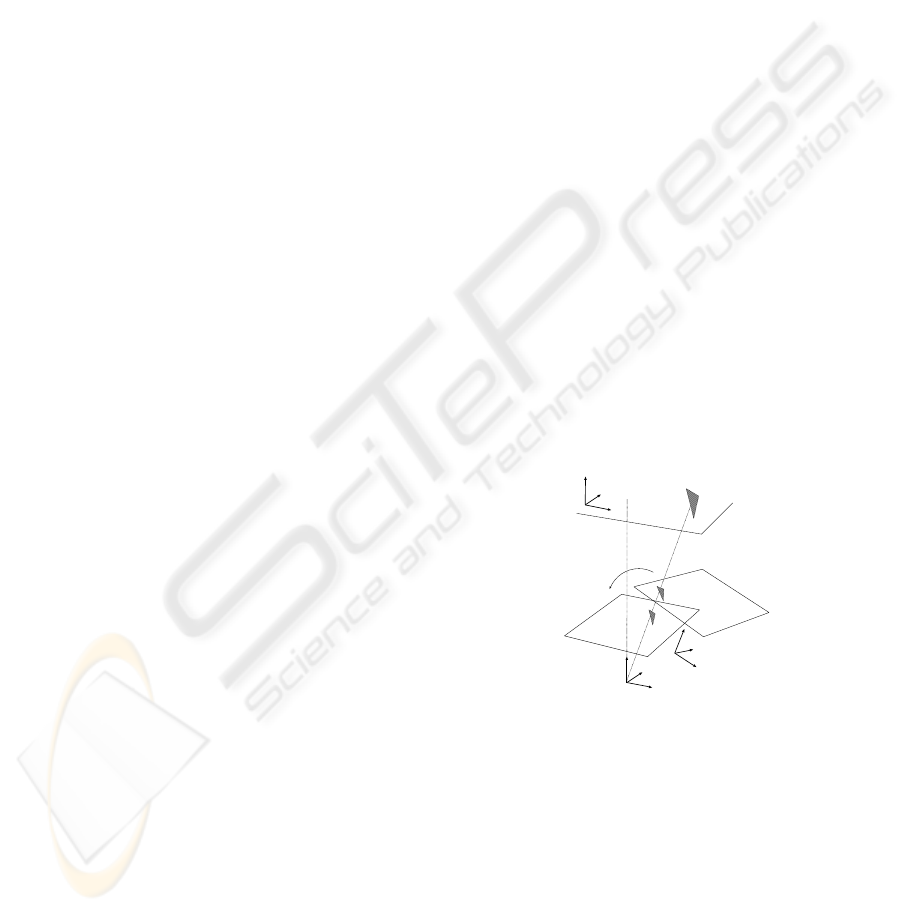
The mobile robot system is composed of three frames

as shown in Figure 1: the world frame F

, the ro-

bot frame F

and the camera frame F

. To localize

the robot in its environnement one have to estimate

the transformation

between the world frame

and the robot frame. Assuming that the transforma-

tion

between the camera frame and the robot

frame is known thanks to a camera-robot calibrating

method, the image is corrected so that it corresponds

to what would be observed if the camera frame ﬁts the

robot frame i.e.

= I. As the visual landmarks

are on the ceilling plane, the correction to apply on

the observed data is a homography

. Knowing

can be expressed as follows:

= K



R − tn



−1

(1)

Where K is the camera intrinsic parameters matrix,

R and t are respectively the rotation matrix and the

translation vector in

, n is the vector normal to

the ceilling plane and d is the distance from the robot

frame to this plane. After applying the computed cor-

rection to image data, one can assume for the clarity

of the presentation and without loss of generality that

is set to the identity matrix.

ceiling Plane

2D pattern

Figure 1: The camera-robot system.

2.2 On-line Robot Pose Computing

Let us denote F

the 2D frame deﬁned by the x and

y-axis of F

and related to the ceiling plane. We

assume that a set of 2D landmarks m

detected on

this plane are modeled and grouped in a mosaic rep-

resented by a set M =





, i = 1, ..., n



where the planar transformation matrix

between

and a frame F

related to m

deﬁnes the pose

of m

in the mosaic (Figure 2). We have

ICINCO 2006 - ROBOTICS AND AUTOMATION

140

(k)

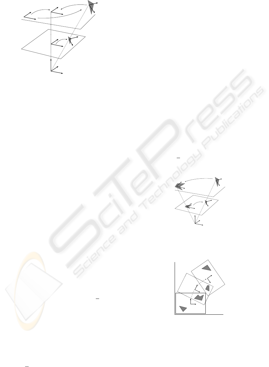
Figure 2: Robot pose computing using visual data of a 2D

model.



0 1



where



Cθ

−Sθ

Sθ

Cθ



expresses the rotation of the model and





its position. Localizing the robot at an in-

stant k consists in computing

(k)

which deﬁnes

the homogenous transformation between the projec-

tion F

(k)

of the camera frame F

on the mosaic plane

as shown in Figure 2. At the instant k, the robot grabs

an image I

of the ceiling. Let F

(k)

be a 2D frame

lied to the image plane. The pose of the projection of

an observed model m

on the image plane is deﬁned

by the transformation

(k)



(k)

0 1



be-

tween F

(k)

and a frame F

(k)

lied to the projection of

where

Cθ

(k)

−Sθ

(k)

Sθ

(k)

Cθ

(k)

express the

rotation of the model and

(k)

its po-

sition in the image. Considering the inverse of the

perspective projection, we obtain the transformation

between the projections F

(k)

and F

of the camera

frame and the model frame respectively on the mo-

saic plane (Figure 1):

(k)



0 1



(k)

0 1

where Z is the distance from the origin of the cam-

era frame to the ceiling and f the focal length. We

can thus express the robot pose relatively to M with

respect to the parameters of a seen model m

(k)



(k)



−1

(2)

Note that the robot position is computed up to a

scale factor

. The absolute position can be retrieved

if the camera is calibrated. Otherwise, the computed

pose is sufﬁcient to achieve navigation using visual

servoing as we will see in section 3.

2.3 Environment Mapping

We will now explain the process of building the mo-

saic of 2D landmarks. At time k = 0, the robot grabs

an image I

, generates a ﬁrst 2D model m

and as-

sociates to it a frame F

. In fact, this ﬁrst model will

serve as a reference to the mosaic. Thus, we have

= F

and

(k)

= I (I is the identity matrix).

In the image I

, a tracker τ

is initialized with a state

(0)

. As the robot moves, the state of τ

evoluates

with respect to k. The system generates other mod-

els. At each generation of a new model m

at the

instant k, a new tracker τ

is initialized with a state

(k)

. Due to the mosaic rigidity, the transforma-

tion between the two model frames is time indepen-

dent and equal to

(k)

(Figure3). Not-

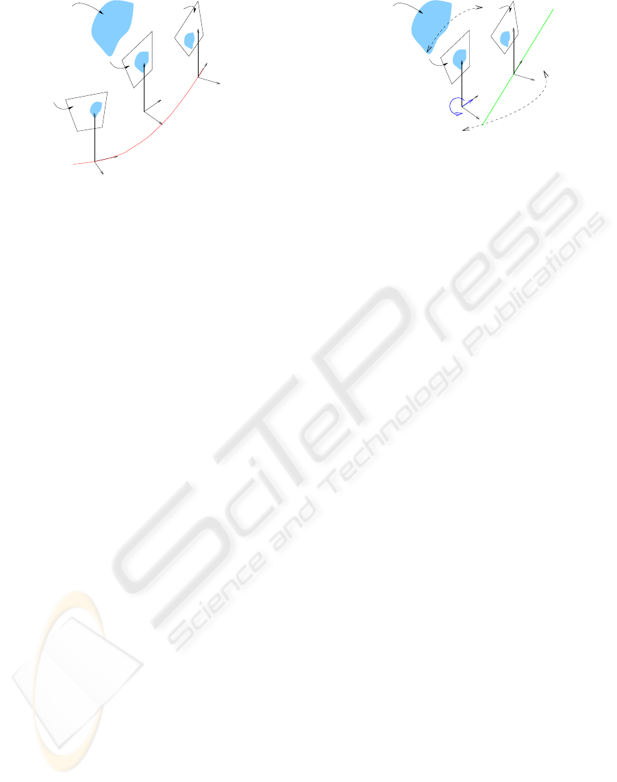
ing



0 1



and projecting this trans-

formation onto the mosaic plane we obtain the pose



0 1



of the new model m

in M:

(k)

Figure 3: Computing the pose of a new model in the mosaic.

Figure 4: An example of key images forming a trajectory.

Of course, as the robot moves, m

may eventually

disappear at an instant k when creating a new model

. In fact, it is sufﬁcient that at least one model m

already deﬁned in the mosaic, is seen at the instant k.

To compute the pose

, we ﬁrst calculate

and

PATTERN TRACKING AND VISUAL SERVOING FOR INDOOR MOBILE ROBOT ENVIRONMENT MAPPING

AND AUTONOMOUS NAVIGATION

141

project it to obtain

. The model m

is then added

to M with the pose

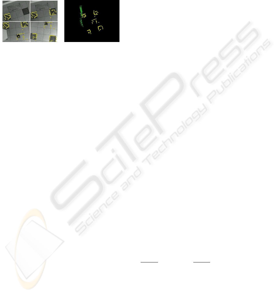
. Figure 5 shows

an example of mosaic construction using the sequence

presented on the left hand side. The set of images rep-

resents the detected 2D models. The right image is a

representation of the constructed mosaic and the robot

locations (gray triangles) during navigation.

(a) (b)

Figure 5: An example of mosaic: (a) a set of key-images

with detected 2D patterns, (b) The mosaic and robot loca-

tions.

2.4 Path Learning and Visual

Navigation

The idea is to enable the robot to learn and repro-

duce some paths joining important places in the en-

vironment. Let us consider a trajectory executed dur-

ing the learning phase and joining a point A to a

point B. A set of so called key images is chosen

among the sequence of video images acquired dur-

ing the learning stage. A key image I

is deﬁned by

a set of mosaic models and their poses in the image

(Figure 4): I

(AB)

n

(k)



, i = 1, 2, ...

. A

trajectory relating A and B is then noticed Φ

(AB)

, k = 1, 2, ...

. Key images are chosen so

that the combination of the elementary trajectories be-

tween each couple of successive key images I

(AB)

and I

(AB)

k+1

forms a global trajectory which approxi-

matively ﬁts the learned trajectory. Some conditions

have to be satisﬁed when creating Φ

: i) two suc-

cessive key images must contain at least one common

model of the mosaic, ii) the variation of the orienta-

tion of a model between two successive key images is

smaller than a deﬁned threshold. The ﬁrst condition

is necessary to visual servoing. The second is moti-

vated by the fact that several different paths joining

two poses do exist. It is thus necessary to insert ad-

ditional key images to reduce the variation of orienta-

tion between two successive images (Figure 4).Visual

servoing is used to carry the robot from a key image

to another.

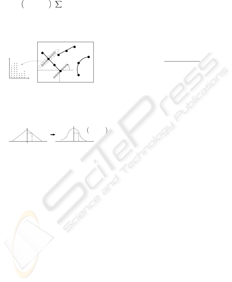
2.5 Pattern Tracking

The tracking problem can be expressed as the es-

timation of the state of a dynamical system basing

on noisy measurements done at discrete times. Let

us consider that, at time k, the state of a system is

deﬁned by a vector X

and the measurements by a

vector Z

. Based on a Bayesian approach, the track-

ing consists in iteratively predicting and updating the

posterior density function (pdf) of the system state

using respectively the dynamical and the observation

models. The pdf p (X

1:k

) is thus estimated as the

vector Z

1:k

= (Z

, i = 1, ..., k) containing the latest

measurements becomes available online.

The tracker developed for this application uses

the condensation algorithm (Isard and Blake, 1998)

which is based on particle ﬁltering theory (Arulam-

palam et al., 2002). First, a pattern model is de-

ﬁned in the image inside an interest window. It is

composed of contours approximated by segments and

arcs. The model contains also a list of vectors whose

elements represent the evolution of image gray scales

in the gradient direction around points sampled on the

contours (Figure 6). Polygonal representation of the

contours is used for automatic pattern generation and

recognition. This enables tracking initialization. Dur-

ing the tracking, only gray scale vectors are used to

estimate the state of the pattern. To formalize this

model, let us consider a window of interest in the im-

age with a center (x

, y

) and dimensions ∆

and ∆

Each segmented contour is sampled in a set of image

points



(j)



(j)

, v

(j)



, j = 1, ..., N



where

is the number of points. At each point, we built a

vector V

(j)



(j)

, g

(j)

, ..., g

(j)

, ...



composed of

gray scale value samples from the image follow-

ing the gradient direction at the pixel m

(j)

and with

a ﬁxed step size δ. g

(j)

is a bilinear approximation

of the gray scale values of the nearest four pixels. A

pattern model can thus be expressed as follows:

M =

n

(j)

, V

(j)

, W

(j)



, j = 1, ..., N

(3)

with U

(j)



(j)

, y

(j)

, φ

(j)



, where x

(j)

−x

∆

and y

(j)

−y

∆

are the normalized co-

ordinates of m

(j)

inside the interest window and

(j)

the gradient orientation at m

(j)

. The vector

(j)



(j)

, b

(j)

, ...



is composed of a set of

parameters deﬁning a function

(j)

which is an ap-

proximation of the one-dimensional discrete normal-

ized auto-correlation function C

(j)

of G

(j)

where

(j)

(l) = g

(j)

for l = 1, ..., N

, and G

(j)

(l) = 0

elsewhere. We have

ICINCO 2006 - ROBOTICS AND AUTOMATION

142

(j)

(λ) = 1/ k V

(j)

l=−N

(j)

(l) G

(j)

(l − λ)

The simplest expression of

(j)

is a straight line

equation (Figure 7). W

(j)

is then one-dimensional

and equal to the slope.

Gray

scale

value

Image

window

(j)

Figure 6: Pattern model: sampled points on segmented con-

tours and corresponding gray scale vectors in the gradient

direction.

(j)

Ω

(j)

(j)−1

(j)

Figure 7: Deriving the probability measure from the inter-

correlation measure.

The state vector X

deﬁnes the pattern pose in im-

age I

at time k :

= (x

, y

, θ

, s

)

(4)

, y

, θ

are respectively the position of the

pattern center and its orientation in the image frame

and s

is the scale factor. The key idea is to use

a Monte Carlo method to represent the pdf of X

by a set of samples (particles) S

(i)

. A weight w

(i)

is associated to each particle. It corresponds to the

probability of realization of the particle. Starting

from a set

(i)

, i = 1, ..., N

of N

particles

with equal weights w

(i)

, the algorithm consists

in iteratively: 1) applying the evolution model on

each particle to make it evolve toward a new state

(i)

k+1

, 2) computing the new weights w

(i)

k+1

using

the observation model, 3) re-sampling the particle

set (particles with small weights are discarded while

particles which obtained high scores are duplicated

so that N

remains constant).

A key point in particle ﬁltering is the deﬁnition

of the observation model Z

in order to estimate

(i)

= p



(i)



. For each predicted particle

(i)

, the model is ﬁtted to the image I

. Around

each image point coinciding with a model point m

an observed vector V

(j)



(j)

, g

(j)

, ..., g

(j)

, ...



of gray scales is built following a direction which is

the transformation of the gradient orientation of the

model. For each observed vector we compute the nor-

malized inter-correlation between the vector stored in

the model and the observed vector components:

(j)

k V

(j)

kk V

(j)

The question is now how to use the inter-correlation

measure to estimate p



(i)



? We ﬁrst com-

pute the probability p



(j)

(i)



that each model

point m

(j)

is placed according to the state vec-

tor particle S

(i)

on the corresponding point in the

observed pattern. The maximum of probability is

expected at m

(j)

. The inter-correlation measure

(j)

(k)

can yeld an estimate of the deviation λ

(j)

(j)−1



(j)



between the observed and the pre-

dicted gray scale vectors,

(j)−1

being the inverse

of the auto-correlation function. Assuming that the

probability that the observed gray scale vector ﬁts the

predicted one follows a Gaussian distribution with re-

spect to λ

(j)

(Figure 7) we can reasonably approx-

imate p



(j)

(i)



by Ω

(λ), the one-dimensional

Gaussian function with standard deviation σ. Assum-

ing that the probabilities p



(j)

(i)



are mutually

independent, it results that



(i)



j=1



(j)

(i)



(5)

more details about handling partial occlusions and

scale changing effects can be found in [*].

3 VISUAL ROUTE FOLLOWING

Visual-servoing is often considered as a way to

achieve positioning tasks. Classical methods, based

on the task function formalism, are based on the exis-

tence of a diffeomorphism between the sensor space

and the robot’s conﬁguration space. Due to the non-

holomic constraints of most of wheeled mobile ro-

bots, under the condition of rolling without slipping,

such a diffeomorphism does not exist if the camera is

rigidly ﬁxed to the robot. In (Tsakiris et al., 1998),

PATTERN TRACKING AND VISUAL SERVOING FOR INDOOR MOBILE ROBOT ENVIRONMENT MAPPING

AND AUTONOMOUS NAVIGATION

143

i+1

Landmark

i+1

Figure 8: Frames and images: I

and I

i+1

are two consec-

utive key images, acquired along a teleoperated path γ.

the authors add extra degrees of freedom to the cam-

era. The camera pose can then be regulated in a closed

loop.

In the case of an embedded and ﬁxed camera, the con-

trol of the camera is generally based on wheeled mo-

bile robots control theory (Samson, 1995). In (Ma

et al., 1999), a car-like robot is controlled with re-

spect to the projection of a ground curve in the im-

age plane. The control law is formalized as a path

following problem. More recently, in (Chen et al.,

2003), a partial estimation of the camera displace-

ment between the current and desired views has been

exploited to design vision-based control laws. A tra-

jectory following task is achieved. The trajectory to

follow is deﬁned by a prerecorded video. In our case,

unlike a whole video sequence, we deal with a set of

relay images which have been acquired from geomet-

rically spaced out points of view.

A visual route following can be considered as a se-

quence of visual-servoing tasks. A stabilization ap-

proach could thus be used to control the camera mo-

tions from a key image to the next one. However, a

visual route is fundamentally a path. To design the

controller, described in the sequel, the key images of

the reference visual route are considered as consec-

utive checkpoints to reach in the sensor space. The

control problem is formulated as a path following to

guide the nonholonomic mobile robot along the visual

route.

3.1 Assumptions and Models

Let I

, I

i+1

be two consecutive key images of a

given visual route to follow and I

be the current

image. Let us note F

= (O

, X

, Y

, Z

) and

i+1

= (O

i+1

, X

i+1

, Y

i+1

, Z

i+1

) the frames at-

tached to the robot when I

and I

i+1

were stored and

= (O

, X

, Y

, Z

) a frame attached to the robot

in its current location. Figure 8 illustrates this setup.

The origin O

of F

is on the axle midpoint of a cart-

i+1

Landmark

i+1

R ,

Figure 9: Control strategy.

like robot, which evolutes on a perfect ground plane.

The control vector of the considered cart-like robot

is u = [V, ω]

where V is the longitudinal veloc-

ity along the axle Y

of F

, and ω is the rotational

velocity around Z

. The hand-eye parameters (i. e.

the rigid transformation between F

and the frame at-

tached to the camera) are supposed to be known.

The state of a set of visual features P

is known

in the images I

and I

i+1

. Moreover P

has been

tracked during the learning step along the path ψ be-

tween F

and F

i+1

. The state of P

is also assumed

available in I

(i.e P

is in the camera ﬁeld of view).

The task to achieve is to drive the state of P

from its

current value to its value in I

i+1

3.2 Principle

Consider the straight line Γ = (O

i+1

, Y

i+1

) (see Fig-

ure 9). The control strategy consists in guiding I

i+1

by regulating asymptotically the axle Y

on Γ.

The control objective is achieved if Y

is regulated to

Γ before the origin of F

reaches the origin of F

i+1

This can be done using chained systems. Indeed in

this case chained system properties are very interest-

ing. A chained system results from a conversion of a

mobile robot non linear model into an almost linear

one (Samson, 1995). As long as the robot longitudi-

nal velocity V is non zero, the performances of path

following can be determined in terms of settling dis-

tance (Thuilot et al., 2002). The settling distance has

to be chosen with respect to robot and perception al-

gorithm performances.

The lateral and angular deviations of F

with re-

spect to Γ to regulate can be obtained through par-

tial Euclidean reconstructions as described in the next

section.

3.3 Evaluating Euclidean State

The tracker presented in Section 2.5 can provide a set

of image points P

= {p

, k = 1 · · · n} belong-

ing to I

i+1

. These points are matched with the set

of image points P

= {p

, k = 1 · · · n} of I

Let Π be a 3D reference plane deﬁned by three 3D

ICINCO 2006 - ROBOTICS AND AUTOMATION

144

points whose projections onto the image plane belong

to P

(and P

). The plane Π is given by the vector

= [n

∗

] in the frame F

i+1

, where n

∗

is the uni-

tary normal of Π in F

i+1

and d

∗

is the distance from

Π to the origin of F

i+1

. It is well known that there is a

projective homography matrix G, relating the image

points of P

and P

(Hartley and Zisserman, 2000):

= Gp

where α

is a positive scaling factor.

Given at least four matched points belonging to Π,

G can be estimated by solving a linear system. If the

plane Π is deﬁned by 3 points, at least ﬁve supplemen-

tary points are necessary to estimate the homography

matrix (Hartley and Zisserman, 2000). Assuming that

the camera calibration K is known, the Euclidean ho-

mography of plane Π is estimated as H = K

−1

and it can be decomposed into a rotation matrix and a

rank 1 matrix: H =

i+1

∗

⊤

∗

. As exposed

in (Faugeras and Lustman, 1988), it is possible from

H to determine the camera motion parameters, that is

i+1

and

i+1

∗

. The normal vector n

∗

can also be

determined, but the results are better if n

∗

has been

previously well estimated (note that it is the case in

indoor navigation with a camera looking at the ceil-

ing for instance). In our case, the mobile robot is sup-

posed to move on a perfect ground plane. Then an

estimation of the angular deviation γ between F

and

i+1

can be directly extracted from

i+1

. Further-

more, we can get out from

i+1

∗

the lateral deviation

z up to a scale factor between the origin of F

and a

straight line Γ (refer to Figure 9).

As a consequence, the control problem can be for-

mulated as following Γ in regulating to zero z and γ

before the origin of F

reaches the origin of F

i+1

3.4 Control Law

Exact linearization of nonlinear models of wheeled

mobile robot under the assumption of rolling without

slipping is a well known theory, which has already

been applied in many vehicle guidance applications,

as in (Thuilot et al., 2002) for a car-like vehicle, and

in our previous works (see [**]). The used state vec-

tor of the robot is Z = [

c z γ

]

⊤

, where c is the

curvilinear coordinate of a point M, which is the or-

thogonal projection of the origin of F

on Γ. The

derivative of this state give the following state space

model:

˙c = V cos γ; ˙z = V sin γ; ˙γ = ω

(6)

The state space model (6) is converted into a chained

system of dimension 3 [

]

⊤

. Deriving

this system with respect to a

gives an almost linear

system. By choosing a

= c and a

= z, and thanks

to classical linear automatics, it is then possible to

design an asymptotically stable guidance control law,

which performances are theoretically independent to

the longitudinal velocity V :

ω(z, γ) = −V cos

γK

z − |V cos

γ|K

tan γ (7)

and K

are gains which set the performances of

the control law. They must be positive for the control

law stability. Their choice determine a settling dis-

tance for the control, i. e. the impulse response of z

with respect to the covered distance by the point M

on Γ.

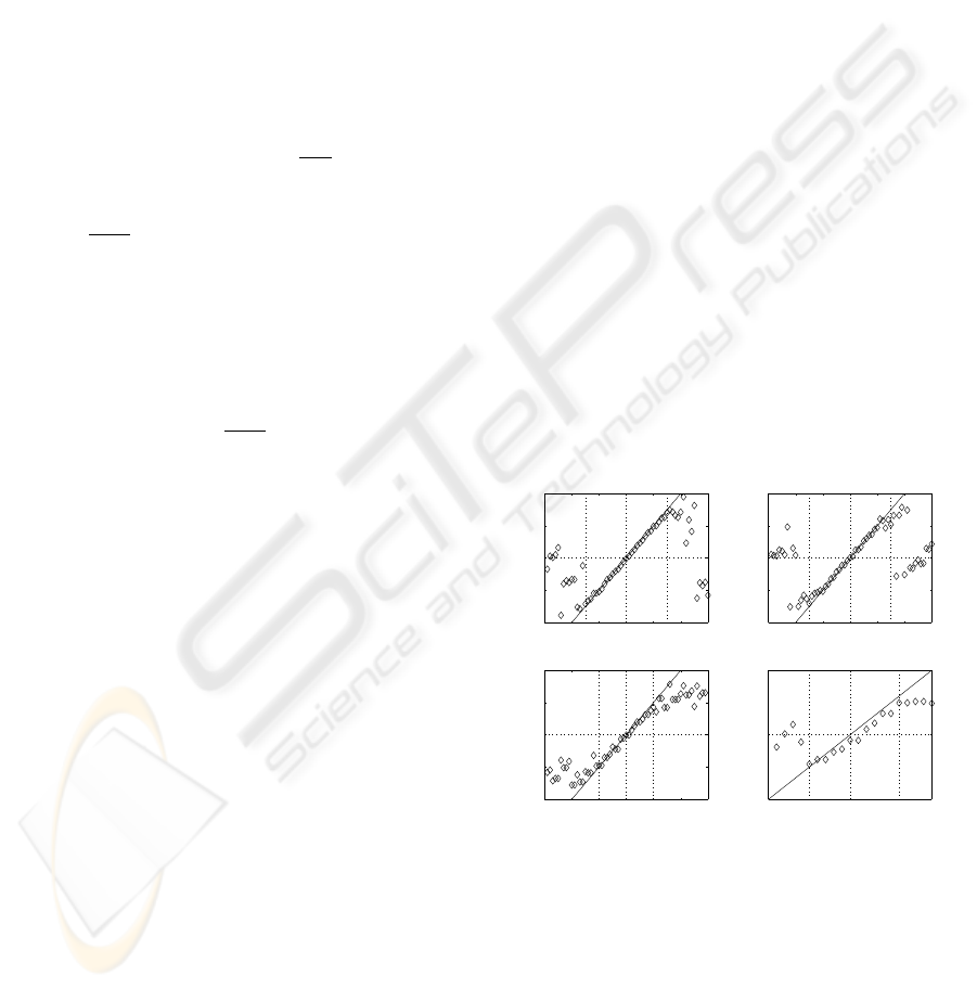
4 EXPERIMENTAL EVALUATION

4.1 Pattern Tracker Evaluation

The evaluation of the tracker was done by superim-

posing an image patch (pattern) with known state vec-

tor trajectory on a cluttered background image se-

quence. The goal was to analyse the accuracy of the

tracker with respect to the pattern displacement mag-

nitude. The number of particles was set to 200 and the

standard deviations of the evolution model parameters

were σ

= 5 pixels, σ

= 3 degrees,

= 0.1. Figure 10 shows displacements and scale

variations estimated by the tracker with respect to the

ground truth values. It can be noticed that the tracker

remains accurate inside [−3σ, +3σ].

−30 −20 −10 0 10 20 30

−20

−10

dX (ground truth)

estimated dX

−30 −20 −10 0 10 20 30

−20

−10

dY (ground truth)

estimated dY

−15 −10 −5 0 5 10 15

−10

−5

dtheta (ground truth)

estimated dtheta

0.5 1 1.5

0.5

1.5

scale (ground truth)

estimated scale

Figure 10: State vector variation estimates (dX and dY in

pixels and dtheta in degrees) with respect to real variation

values (The straight line represents the ideal curve).

4.2 A Navigation Task

The proposed framework is implemented on a

Pekee

robot which is controlled from an external

PC. A small 1/3” CMOS camera is embedded on the

robot and looks at the ceiling which is generally a

PATTERN TRACKING AND VISUAL SERVOING FOR INDOOR MOBILE ROBOT ENVIRONMENT MAPPING

AND AUTONOMOUS NAVIGATION

145

plane parallel to the ground. Then, it is quite easy to

give a good approximation of the normal vector n

∗

the reference plane Π in order to evaluate an homog-

raphy. If the camera frame is confounded with the ro-

bot frame F

, we can assume that n

∗

= [

0 0 1

The displacement between F

i+1

and F

only consists

of one rotation γZ

and two translations t

and

Y c

. Therefore, H has only three degrees of free-

dom. Only two points lying on Π and matched in I

i+1

and I

are theoretically necessary to estimate H. The

angular deviation γ and the lateral deviation z with re-

spect to Γ can be estimated directly from the compu-

tation of H. The Figure 12 illustrates the evolution of

planar patterns tracked during the robot motion along

a given visual route. These tracked planar patterns

have been extracted while the user was creating a vi-

sual path which is included into the visual route to be

followed.

At the ﬁrst step of an autonomous run, the current

camera image has to be located into the visual mem-

ory. The tracking of learnt planar pattern in this image

is then automatic. As a consequence, the user must

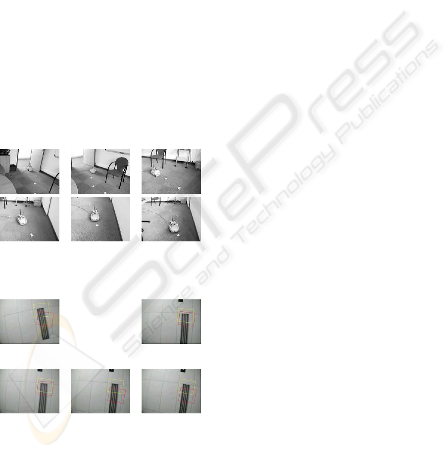
Figure 11: Following a visual route: the previously learnt

visual path, about 10m long, is materialized on the ground.

The pictures were taken during an autonomous run.

(1) [...] (2)

(3) (4) (5)

Figure 12: Evolution of the image when the robot is regu-

lated between two consecutive key image : in each image,

the yellow square is the current state of the tracker, the red

one is the state to reach. The image (3) is considered close

enough to the key image: the control has succeeded. At im-

age (4), a new reference state to reach is then provided to

the control law.

have chosen at least one reference attitude of the ro-

bot which has to be associated with one key image. If

the robot has ever achieved a mission since it has been

started up, the current image is already supposed to

be closed to a key image. At each frame, the tracker

provides the coordinates of a current tracked planar

pattern. H is then computed thanks to the knowledge

of this pattern in the key image to reach I

i+1

. A key

image is assumed to be reached when a distance be-

tween the current points coordinates and the desired

one goes under a ﬁxed threshold. The reference path,

which is represented on the Figure 11 by the white

squares which are lying on the ground, has been ac-

quired as a visual route of ﬁfteen key images. The

corresponding path length is about 10m. The longi-

tudinal velocity V was ﬁxed to 0.2m.s

−1

. When the

robot stops at the end of the visual route, the ﬁnal er-

rors in the image corresponds to a positioning error

around 5cm and an angular error about 3

◦

. Neverthe-

less, note that the robot has been stopped roughly, by

setting V to zero since the last key image of the vi-

sual route has been detected. Moreover, both camera

intrinsic and hand-eye parameters has been roughly

determined. The positioning accuracy depends above

all on the threshold which determines if a key image

is reached. Our future works will improve that point.

5 CONCLUSION

An efﬁcient particle ﬁlter tracker with speciﬁc obser-

vation probability densities was designed to track pla-

nar modelled patterns on cluttered background. Scale

changing and partial occlusions were taken into ac-

count. The obtained algorithm runs in near real time

rate and is accurate and robust in realistic conditions

according to experimental validation. The tracker

was used for autonomous indoor environment map-

ping and image-based navigation. Visual route is per-

formed thanks to a visual-servoing control law, which

is adapted to the robot nonholonomy. Experimental

results conﬁrm the validity of the approach. Future

works will deal with the adaptation of the tracker to

3D movement tracking using homographies in order

to enable autonomous mapping of 3D indoor environ-

ment using planar patterns detected on the walls.

REFERENCES

Arulampalam, S., Maskell, S., Gordon, N., and Clapp, T.

(2002). A tutorial on particle ﬁlters for on-line non-

linear/non-gaussian bayesian tracking. IEEE Trans.

on Signal Processing, 50:174–188.

Bascle, B., Bouthemy, P., Deriche, R., and Meyer, F. (1994).

Tracking complex primitives in an image sequence. In

ICINCO 2006 - ROBOTICS AND AUTOMATION

146

In Proc. of the 12th int. Conf. on Pattern Recognition,

pages 426–431.

Black, M. and Jepson, A. (1996). Eigentracking: robust

matching and tracking of articulated objects using

a view-based representation. In In Proc. European

Conf. on Computer Vision, pages 329–42.

Blake, A., Curwen, R., and Zisserman, A. A. (1993). A

framework for spatiotemporal control in the tracking

of visual contours. Int. J. Computer Vision, 11:127–

145.

Chen, J., Dixon, W. E., Dawson, D. M., and McIntire, M.

(2003). Homography-based visual servo tracking con-

trol of a wheeled mobile robot. In Proceeding of the

2003 IEEE/RSJ Intl. Conference on Intelligent Robots

and Systems, pages 1814–1819, Las Vegas, Nevada.

Fang, Y., Dawson, D., Dixon, W., and de Queiroz,

M. (2002). Homography-based visual servoing of

wheeled mobile robots. In Conference on Decision

and Control, pages 2866–2871, Las Vegas, NV.

Faugeras, O. and Lustman, F. (1988). Motion and structure

from motion in a piecewise planar environment. Int.

Journal of Pattern Recognition and Artiﬁcial Intelli-

gence, 2(3):485–508.

Hartley, R. and Zisserman, A. (2000). Multiple View Geom-

etry in Computer Vision. Cambridge University Press.

Hayet, J. (2003). Contribution

a la navigation d’un robot

mobile sur amers visuels textur

es dans un environ-

nement structur

e. PhD thesis, Universit Paul Sabatier,

Toulouse.

Isard, M. and Blake, A. (1998). Condensation-conditional

density propagation for visual tracking. Int. J. Com-

puter Vision, 29:5–28.

Jurie, F. and Dhome, M. (2001). Real-time template match-

ing: an efﬁcient approach. In In the 12th Int. Conf. on

Computer Vision, Vancouver.

Kass, M., Witkin, A., and Terzopoulos, D. (1988). Snakes:

active contours. Int. J. Computer Vision, 1:321–331.

Lowe, D. (1992). Robust model-based motion tracking

through the integration of search and estimation. Int.

J. Computer Vision, 8:113–122.

Ma, Y., Kosecka, J., and Sastry, S. S. (1999). Vision guided

navigation for a nonholonomic mobile robot. IEEE

Transactions on Robotics and Automation, pages 521–

37.

Malis, E., Chaumette, F., and Boudet, S. (1999). 2 1/2 d

visual servoing. IEEE Transactions on Robotics and

Automation, 15(2):238–250.

Marchand, E., Bouthemy, P., Chaumette, F., and Moreau, V.

(1999). Robust real-time visual tracking using a 2d-3d

model-based approach. In In Proc. IEEE Int. Conf. on

Computer Vision, ICCV’99, pages 262–268, Kerkira,

Greece.

Pece, A. E. C. and Worrall, A. D. (2002). Tracking with

the em contour algorithm. In In Proc. of the European

Conf. on Computer Vision, pages 3–17, Copenhagen,

Danemark.

Samson, C. (1995). Control of chained systems. applica-

tion to path following and time-varying stabilization

of mobile robots. IEEE Transactions on Automatic

Control, 40(1):64–77.

Se, S., Lowe, D., and Little, J. (2001). Vision-based mobile

robot localization and mapping using scale invariant

features. In Int. Conference on Robotics and Automa-

tion (ICRA’01).

Talluri, R. and Aggarwal, J. (1996). Mobile robot self-

location using model-image feature correspondence.

IEEE Trans. on Robotics and Automation, 12(1):63–

77.

Thuilot, B., Cariou, C., Martinet, P., and Berducat, M.

(2002). Automatic guidance of a farm tractor relying

on a single cp-dgps. Autonomous Robots, 13:53–71.

Tsakiris, D., Rives, P., and Samson, C. (1998). Extend-

ing visual servoing techniques to nonholonomic mo-

bile robots. In D. Kriegman, G. H. and Morse, A., ed-

itors, The Conﬂuence of Vision and Control, volume

237 of LNCIS, pages 106–117. Springer Verlag.

Zhong, Y., Jain, A. K., and Dubuisson, M. P. (2000). Object

tracking using deformable templates. IEEE Trans. on

Pattern Analysis and Machine Intelligence, 22:544–

549.

PATTERN TRACKING AND VISUAL SERVOING FOR INDOOR MOBILE ROBOT ENVIRONMENT MAPPING

AND AUTONOMOUS NAVIGATION

147