THE LAGR PROJECT
Integrating Learning into the 4D/RCS Control Hierarchy
James Albus, Roger Bostelman, Tsai Hong, Tommy Chang, Will Shackleford, Michael Shneier
National Institute of Standards and Technology, 100 Bureau Drive, Gaithersburg, MD 20899, USA
Keywords: LAGR, Learning, 4D/RCS, mobile robot, hierarchical control, reference model architecture.
Abstract: The National Institute of Standards and Technology’s (NIST) Intelligent Systems Division (ISD) is a par-
ticipant the Defense Advanced Research Project Agency (DARPA) LAGR (Learning Applied to Ground
Robots) Project. The NIST team’s objective for the LAGR Project is to insert learning algorithms into the
modules that make up the 4D/RCS (Four Dimensional/Real-Time Control System), the standard reference
model architecture to which ISD has applied to many intelligent systems. This paper describes the 4D/RCS
structure, its application to the LAGR project, and the learning and mobility control methods used by the
NIST team’s vehicle.
1 INTRODUCTION
The National Institute of Standards and Technol-
ogy’s (NIST) Intelligent Systems Division (ISD) has
been developing the RCS (Albus-1, 2002; Albus-2,
2002) reference model architecture for over 30
years. 4D/RCS is the most recent version of RCS
developed for the Army Research Lab Experimental
Unmanned Ground Vehicle program. The 4D in
4D/RCS signifies adding time as another dimension
to each level of the three dimensional (sensor proc-
essing, world modeling, behavior generation), hier-
archical control structure. ISD has studied the use of
4D/RCS in defense mobility (Balakirsky, 2002),
transportation (Albus, 1992), robot cranes (Bostel-
man, 1996), manufacturing (Shackleford, 2000;
Michaloski, 1986) and several other applications.
In the past year, ISD has been applying 4D/RCS
to the DARPA LAGR program (Jackel, 2005). The
DARPA LAGR program aims to develop algorithms
that enable a robotic vehicle to travel through com-
plex terrain without having to rely on hand-tuned
algorithms that only apply in limited environments.
The goal is to enable the control system of the vehi-
cle to learn which areas are traversable and how to
avoid areas that are impassable or that limit the mo-
bility of the vehicle. To accomplish this goal, the
program provided small robotic vehicles to each of
the participants (Figure 1). The vehicles are used by
the teams to develop software and a separate
DARPA team, with an identical vehicle, conducts
tests of the software each month. Operators load the
software onto an identical vehicle and command the
vehicle to travel from a start waypoint to a goal
waypoint through an obstacle-rich environment.
They measure the performance of the system on
multiple runs, under the expectation that improve-
ments will be made through learning.
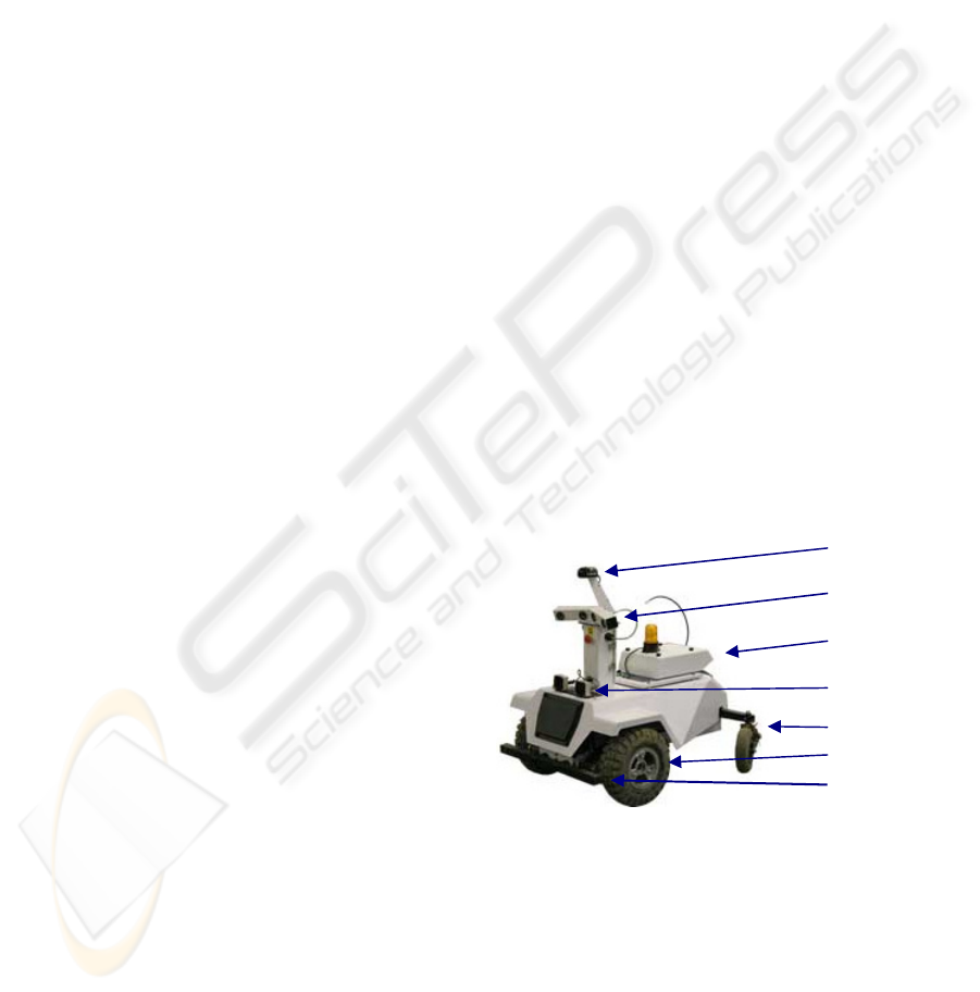
Figure 1: The DARPA LAGR vehicle.
The vehicles are equipped with four computer
processors (right and left cameras, control, and the
planner); wireless data and emergency stop radios;
GPS receiver; inertial navigation unit; dual stereo
cameras; infrared sensors; switch-sensed bumper;
front wheel encoders; and other sensors listed later
in the paper.
Section 2 of this paper describes the 4D/RCS
Reference Model Architecture followed by a more
GPS
A
ntenna
Dual stereo
cameras
Computers,
IMU inside
Infrared
sensors
Casters
Drive wheels
Bumper
154
Albus J., Bostelman R., Hong T., Chang T., Shackleford W. and Shneier M. (2006).
THE LAGR PROJECT - Integrating Learning into the 4D/RCS Control Hierarchy.
In Proceedings of the Third International Conference on Informatics in Control, Automation and Robotics, pages 154-161
DOI: 10.5220/0001210701540161
Copyright
c
SciTePress
specific description of the 4D/RCS application to the
DARPA LAGR Program in Sections 3. Sections 4
include a summary and conclusion.
2 4D/RCS REFERENCE MODEL
ARCHITECTURE
The 4D/RCS architecture is characterized by a ge-
neric control node at all the hierarchical control lev-
els. The 4D/RCS hierarchical levels are scalable to
facilitate systems of any degree of complexity. Each
node within the hierarchy functions as a goal-driven,
model-based, closed-loop controller. Each node is
capable of accepting and decomposing task com-
mands with goals into actions that accomplish task
goals despite unexpected conditions and dynamic
perturbations in the world.
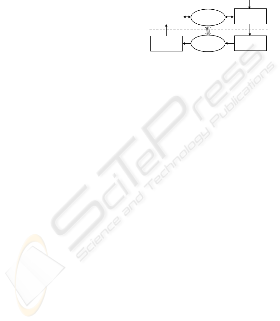
At the heart of the control loop through each
node is the world model, which provides the node
with an internal model of the external world (Figure
2). The world model provides a site for data fusion,
acts as a buffer between perception and behavior,
and supports both sensory processing and behavior
generation.
In support of behavior generation, the world
model provides knowledge of the environment with
a range and resolution in space and time that is ap-
propriate to task decomposition and control deci-
sions that are the responsibility of that node.
A world modeling process maintains the knowl-
edge database and uses information stored in it to
generate predictions for sensory processing and
simulations for behavior generation. Predictions are
compared with observations and errors are used to
generate updates for the knowledge database. Simu-
lations of tentative plans are evaluated by value
judgment to select the “best” plan for execution.
Predictions can be matched with observations for
recursive estimation and Kalman filtering. The
world model also provides hypotheses for gestalt
grouping and segmentation. Thus, each node in the
4D/RCS hierarchy is an intelligent system that ac-
cepts goals from above and generates commands for
subordinates so as to achieve those goals.
The centrality of the world model to each con-
trol loop is a principal distinguishing feature be-
tween 4D/RCS and behaviorist architectures. Be-
haviorist architectures rely solely on sensory feed-
back from the world. All behavior is a reaction to
immediate sensory feedback. In contrast, the
4D/RCS world model integrates all available knowl-
edge into an internal representation that is far richer
and more complete than is available from immediate
sensory feedback alone. This enables more sophisti-
cated behavior than can be achieved from purely
reactive systems.
Perception
Behavior
World Model
Sensing
Action Real World
internal
external
Mission Goal
Figure 2: The fundamental structure of a 4D/RCS control
loop.
The nature of the world model distinguishes
4D/RCS from conventional artificial intelligence
(AI) architectures. Most AI world models are purely
symbolic. In 4D/RCS, the world model is a combi-
nation of instantaneous signal values from sensors,
state variables, images, and maps that are linked to
symbolic representations of entities, events, objects,
classes, situations, and relationships in a composite
of immediate experience, short-term memory, and
long-term memory. Real-time performance in mod-
eling and planning is achieved by restricting the
range and resolution of maps and data structures to
what is required by the behavior generation module
at each level. Short range and high resolution maps
are implemented in the lowest level, with longer
range and lower resolution maps at the higher level.
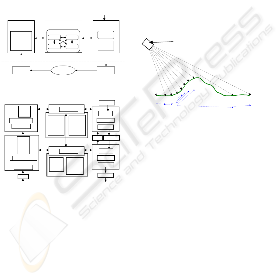
A high level diagram of the internal structure of
the world model and value judgment system is
shown in Figure 3. Within the knowledge database,
iconic information (images and maps) are linked to
each other and to symbolic information (entities and
events). Situations and relationships between enti-
ties, events, images, and maps are represented by
pointers. Pointers that link symbolic data structures
to each other form syntactic, semantic, causal, and
situational networks. Pointers that link symbolic
data structures to regions in images and maps pro-
vide symbol grounding and enable the world model
to project its understanding of reality onto the physi-
cal world.
3 4D/RCS APPLIED TO LAGR
The 4D/RCS architecture for LAGR (Figure 4) con-
sists of only two levels requiring plans at each low
and high level out to approximately 10 m and 100 m,
respectively, in front of the vehicle. This is because
THE LAGR PROJECT - Integrating Learning into the 4D/RCS Control Hierarchy
155
the size of the LAGR test areas is small (typically
about 100 m on a side, and the test missions are
short in duration (typically less than 4 minutes.) For
controlling an entire battalion of autonomous vehi-
cles, there may be as many as five or more 4D/RCS
hierarchical levels.
The following sub-sections describe the type of
algorithms implemented in sensor processing, world
modeling, and behavior generation, as well as a sec-
tion that describes the learning algorithms that have
been implemented.
SENSORY
PROCESSING
WORLD MODELING
VALUE JUDGMENT
KNOWLEDGE
Images
Maps Entities
Sensors
ActuatorsWorld
Classification
Estimation
Computation
Grouping
Windowing
Mission (Goal)
internal
external
Events
Planners
Executors
Task
Knowledge
BEHAVIOR
GENERATION
Figure 3: The basic internal structure of a 4D/RCS control
loop.
SP2
SP1
BG2
Planner2
Executor2
10 step plan
Group pixels
Classify objects
images
name
class
images
color
range
edges
class
Classify pixels
Compute attributes
maps
cost
objects
terrain
200x200 pix
400x400 m
frames
names
attributes
state
class
relations
WM2
Manage KD2
maps
cost
terrain
200x200 pix
40x40 m
state vari-
ables
names
values
WM1
Manage KD1
BG1
Planner1
Executor1
10 step plan
Sensors
Cameras, INS, GPS, bumper, encoders, current
Actuators
Wheel motors, camera controls
Scale & filter
signals
status commands
commands
commands
SP2
SP1
BG2
Planner2
Executor2
10 step plan
Group pixels
Classify objects
images
name
class
images
color
range
edges
class
Classify pixels
Compute attributes
maps
cost
objects
terrain
200x200 pix
400x400 m
frames
names
attributes
state
class
relations
WM2
Manage KD2
maps
cost
objects
terrain
200x200 pix
400x400 m
frames
names
attributes
state
class
relations
WM2
Manage KD2
maps
cost
terrain
200x200 pix
40x40 m
state vari-
ables
names
values
WM1
Manage KD1
maps
cost
terrain
200x200 pix
40x40 m
state vari-
ables
names
values
WM1
Manage KD1
BG1
Planner1
Executor1
10 step plan
Sensors
Cameras, INS, GPS, bumper, encoders, current
Actuators
Wheel motors, camera controls
Scale & filter
signals
status commands
commands
commands
Figure 4: Two-level instantition of the 4D/RCS hierarchy
for LAGR.
3.1 Sensory Processing
The sensor processing column in the 4D/RCS hier-
archy for LAGR (Figure 4) starts with the sensors on
board the LAGR vehicle. Sensors used in the sen-
sory processing module include the two pairs of ste-
reo color cameras, the physical bumper and infra-red
bumper sensors, the motor current sensor (for terrain
resistance), and the navigation sensors (GPS, wheel
encoder, and INS). Sensory processing modules in-
clude a stereo obstacle detection module, a bumper
obstacle detection module, an infrared obstacle de-
tection module, an image classification module, and
a terrain slipperyness detection module.
3.2 Stereo Vision
Stereo vision is primarily used for detecting obsta-
cles. We use the SRI Stereo Vision Engine (Kono-
lige, 2005) to process the pairs of images from the
two stereo camera pairs. For each newly acquired
stereo image pair, the obstacle detection algorithm
processes each vertical scan line in the reference
image independently and classifies each pixel as
GROUND, OBSTACLE, SHORT_OBSTACLE, COVER
or INVALID. Figure 5 illustrates the basic obstacle
detection algorithm (
Chang, 1999).
1
2
3
4
5
6
7
8
9
2
3
4
5
6
7
8
9
0
1
0
Figure 5: A single vertical scanline detecting the ground.
Pixel 0 is altered to correspond to the bottom of the vehi-
cle wheel. Pixels 1, 2, 3, 8 and 9 are ground pixels due to
shallow slopes. Pixel 4, 5, 6 and 7 are obstacles due to
steeper slopes. The slopes are shown by the direction
vectors on the bottom of the figure.
Pixels that are not in the 3D point cloud are
marked INVALID. Pixels corresponding to obstacles
that are shorter than 5 cm high are marked as
SHORT_OBSTACLE. The obstacle height threshold
value of 5cm was chosen such that the LAGR vehi-
cle can ignore and drive over small pebbles and
rocks. Similarly,
COVER corresponds to obstacles
that are taller than 1.5 m, a safe clearance height for
the LAGR vehicle.
Within each reference image, the corresponding
3D points are accumulated onto a 2D cost map of 20
cm by 20 cm cell resolution. Each cell has a cost
value representing the percentage of
OBSTACLE
pixels in the cell. In addition to cost value, color and
elevation statistics are also kept and updated in each
cell. This map is sent the world model at the current
level and to the sensory processing module at the
level above in the 4D/RCS hierarchy.
Figure 6 shows a view of obstacle detection
from the operator control unit (OCU). The vehicle is
shown driving on a dirt road lined with trees with an
200
ms
20
ms
dual stereo cameras
ICINCO 2006 - ROBOTICS AND AUTOMATION
156
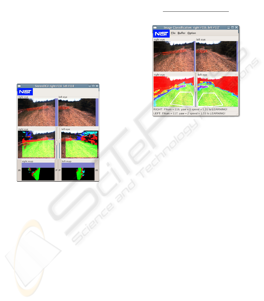
orange fence in the background.
3.3 Learning Classification in Color
Vision
A color-based image classification (Tan, 2006) mod-
ule runs independently from the obstacle detection
module in the lower-level sensory processing mod-
ule. It learns to classify objects in the scene by their
color and appearance. This enables it to provide
information about obstacles and ground points even
when stereo is not available. A flat world assumption
is used when determining the 3D location of a pixel
in the image. This assumption is valid for points
close to the vehicle providing that the vehicle does
not get too close to an obstacle.
Figure 6: OCU display showing original images (top),
results of obstacle detection (middle), and cost maps (bot-
tom). Red represents obstacles, green is ground, and blue
represents obstacles too far away to classify.
Pixels near the vehicle, as defined by a 1 m
wide by 2 m long rectangular area in front of the
vehicle, are used to construct and update the
GROUND color histogram. Similarly, the BACK-
GROUND color histogram is constructed and up-
dated from pixel locations that were previously be-
lieved to be background.
The construction of the background model ini-
tially randomly samples the area above the horizon.
Once the algorithm is running, the algorithm ran-
domly samples pixels in the current frame that the
previous result identified as background. These
samples are used to update the background color
model using temporal fusion
In order to remember multiple color distribu-
tions, multiple GROUND color histograms are
maintained. However, only one BACKGROUND
color histogram is used.
The cost for each pixel is determined by a color
voting method and the degree of belief that a point is
a background is calculated from the two histograms
as
N
BACKGROUND
N
BACKGROUND
N
GROUND
Figure 7: OCU display showing original images (top) and
cost images (bottom). The 1 m wide by 2 m long rectan-
gular areas assumed to be ground (white boxes) are over-
laid on the cost images.
Where N
BACKGROUND
and N
GROUND
are the number of
hits in the corresponding histogram bin. In the case
of multiple GROUND color histograms, the mini-
mum cost is used. The cost image is sent to the
world model. Figure 7 illustrates color classification
on the same image as shown in Figure 6
3.4 World Modeling
The world model is the system's internal representa-
tion of the external world. It acts as a bridge between
sensory processing and behavior generation in the
4D/RCS hierarchy by providing a central repository
for storing sensory data in a unified representation.
It decouples the real-time sensory updates from the
rest of the system. The world model process has two
primary functions: To create a knowledge database
and keep it current and consistent, and to generate
predictions of expected sensory input.
For the LAGR project, two world model levels
have been built (WM1 and WM2). Each world
model process builds a two dimensional (200 x 200
cells) map, but at different resolutions. These are
used to temporally fuse information from sensory
processing. Currently the lower level (SP1) is fused
into both WM1 and WM2 as the learning module in
THE LAGR PROJECT - Integrating Learning into the 4D/RCS Control Hierarchy
157
SP2 does not yet send its models to WM. Figure 8
shows the WM1 and WM2 maps constructed from
the stereo obstacle detection module in SP1. The
maps contain traversal costs for each cell in the map.
The position of the vehicle is shown as an overlay
on the map. The red, yellow, blue, light blue, and
green are cost values ranging from high to low cost,
and black represents unknown areas. Each map cell
represents an area on the ground of a fixed size and
is marked with the time it was last updated. The total
length and width of the map is 40 m for WM1 and
120 m for WM2. The information stored in each cell
includes the average ground and obstacle elevation
height, the variance, minimum and maximum height,
and a confidence measure reflecting the "goodness"
of the elevation data. In addition, a data structure
describing the terrain traversability cost and the cost
confidence as updated by the stereo obstacle detec-
tion module, image classification module, bumper
module, infrared sensor module, etc. The map updat-
ing algorithm is based on confidence-based mapping
as described in (Oskard, 1990). The costs and the
confidences are combined to determine the relative
safety of traversing the grid with the following equa-
tion:
tionclassificac
lagrLearnlstereoscell
CostW
CostWCostWCost
×
+
×+×=
where Cost
cell
is the cost to traverse each grid
cell. Cost
lagrLearn
, Cost
classification
, and Cost
stereo
are the
fused costs in the world model based on the learning
module, classification module, stereo obstacle detec-
tion module. W
s
, W
l
, and W
c
are weighting con-
stants for each cost. However, Cost
cell
is a bumper
cost if there is a bumper hit.
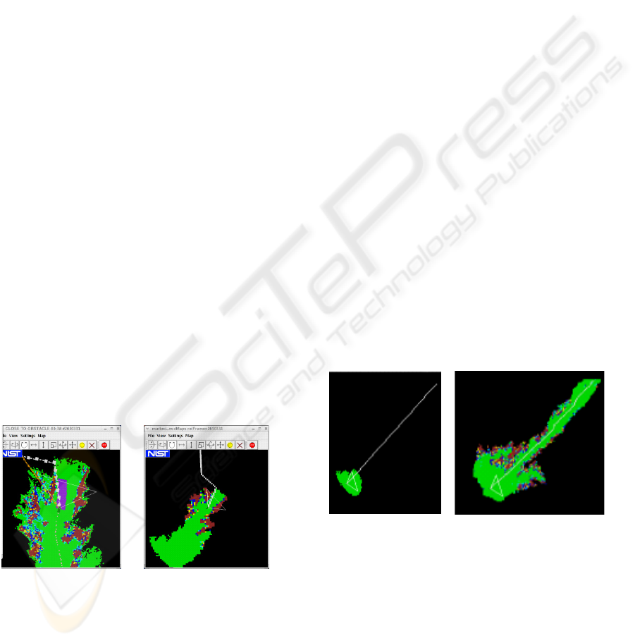
Figure 8: OCU display of the World Model cost maps built
from sensor processing data. WM1 builds a 0.2 m resolu-
tion cost map (left) and WM2 builds a 0.6 m resolution
cost map (right).
The final cost placed in each map cell represents
the best estimate of terrain traversability in the re-
gion represented by that cell, based on information
fused over time. Each cost has a confidence associ-
ated with it and the map grid selects the label with
the highest confidence. The final cost maps are con-
structed by taking the fused cost from all the sensory
processing modules.
Efficient functions have been developed to
scroll the maps as the vehicle moves, to update map
data, and to fuse data from the sensory processing
modules. A map is updated with new sensor data and
scrolled to keep the vehicle centered. This minimizes
grid relocation. No copying, only updating, of data is
done. When the vehicle moves out of the center grid
cell of the map, the scrolling function is enabled.
The map is vehicle-centered, so only the borders
need to be initialized. Initialization information may
be obtained from remembered maps saved from pre-
vious test runs as shown in Figure 9. Remembering
maps is a very effective way of learning about ter-
rain, and has proved important in optimizing succes-
sive runs over the same terrain.
The cost and elevation confidence of each grid
cell is updated every sensor cycle: 5 Hz for the ste-
reo obstacle detection module, 3 Hz for the learning
module, 5 Hz for the classification module, and 10-
20 Hz for the bumper module. The confidence val-
ues are used as a cost factor in determining the
traversability of a cell.
We plan additional research to implement mod-
eling of moving objects (cars, targets, etc.) and to
broaden the system's terrain and object classification
capabilities. The ability to recognize and label water,
rocky roads, buildings, fences, etc. would enhance
the vehicle's performance.
Figure 9: Initial (left) and remembered (right) cost maps as
the system starts without and with saved maps, respec-
tively.
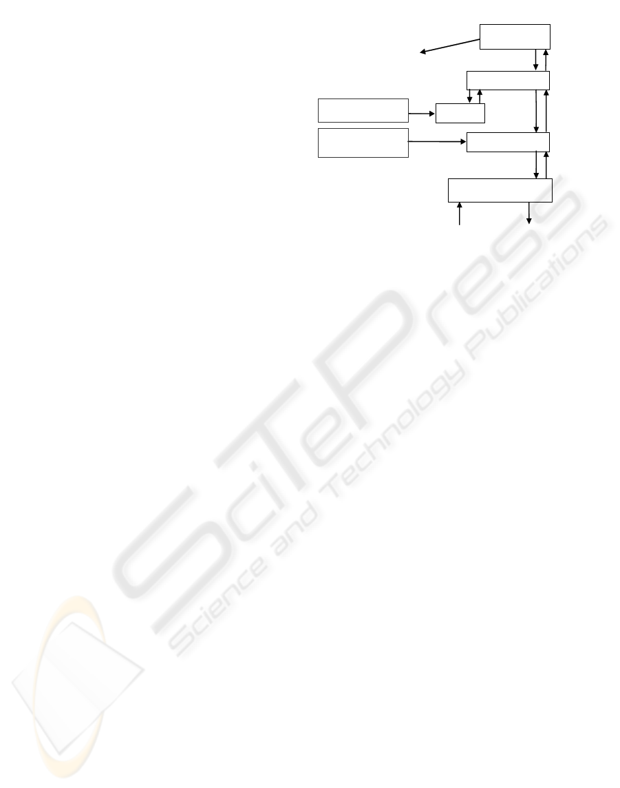
3.5 Behavior Generation
Top level input to Behavior Generation (BG) (Figure
10) is a file containing the final goal point in UTM
(Universal Transverse Mercator) coordinates. At the
bottom level in the 4D/RCS hierarchy, BG produces
a speed for each of the two drive wheels updated
every 20 ms, which is input to the low-level control-
ICINCO 2006 - ROBOTICS AND AUTOMATION
158
ler included with the government-provided vehicle.
The low-level system returns status to BG, including
motor currents, position estimate, physical bumper
switch state, raw GPS and encoder feedback, etc
These are used directly by BG rather than passing
them through sensor processing and world modeling
since they are time-critical and relatively simple to
process.
Two position estimates are used in the system.
Global position is strongly affected by the GPS an-
tenna output and is more accurate over long ranges,
but can be noisy. Local position uses only the wheel
encoders and inertial measurement unit (IMU). It is
less noisy than GPS but drifts significantly as the
vehicle moves, and even more if the wheels slip.
The system consists of five separate executa-
bles. Each sleeps until the beginning of its cycle,
reads its inputs, does some planning, writes its out-
puts and starts the cycle again. Processes communi-
cate using the Neutral Message Language (NML) in
a non-blocking mode, which wraps the shared-
memory interface (
Shackleford, 1990). Each module
also posts a status message that can be used by both
the supervising process and by developers via a di-
agnostics tool to monitor the process.
The LAGR Supervisor is the highest level BG
module. It is responsible for starting and stopping
the system. It reads the final goal and sends it to the
waypoint generator. The waypoint generator chooses
a series of waypoints for the lowest-cost traversable
path to the goal using global position and translates
the points into local coordinates. It generates a list of
waypoints using either the output of the A* Planner
(
Heyes-Jones, 2005) or a previously recorded known
route to the goal.
The planner takes a 201 X 201 terrain grid from
WM, classifies the grid, and translates it into a grid
of costs of the same size. In most cases the cost is
simply looked up in a small table from the corre-
sponding element of the input grid. However, since
costs also depend on neighboring costs, they are
automatically adjusted to allow the vehicle to con-
tinue motion.
Lagr Superviso
r
Waypoint Generato
r
A
* Planne
r
Waypoint Followe
r
LAGR CMU Comm Interface
Final Goal (UTM Easting,Northing)
List of waypoints
local coordinates
{(x,y), …, (x,y)}
velocity and
heading
wheel speed
s
p
osition,motor current,
bumper, etc.
Long range (120m)
Low resolution (0.6m) Map
Clear/Save Map
s
Short range (40m)
High resolution (0.2m)
Map
Behavior Generation World Modeling
Figure 10: Behavior Generation High Level Data Flow
Diagram.
The waypoint follower receives a series of way-
points, spaced approximately 0.6 m apart that could
be used to drive blindly without a map. However,
there are some features of the path that make this
less than optimal. When the path contains a turn, it
is either at a 0.8 rad (45 degree) or 1.6 rad (90 de-
gree) angle with respect to the previous heading. The
waypoint follower could smooth the path, but it
would at least partially, enter cells that were not
covered by the path chosen at the higher level. The
A* planner might also plan through a cell that was
partially blocked by an obstacle. The waypoint fol-
lower is then responsible for avoiding the obstacle.
The first step in creating a short range plan is to
choose a goal point from the list provided by the A*
Planner. One option would be to use the point where
the path intersects the edge of the 40m map. How-
ever, due to the differences between local and global
positioning, this point might be on one side of an
obstacle in the long range map and on the other side
in the short range map. To avoid this, the first major
turning point is selected. The waypoint follower
searches a preset list of possible paths starting at the
current position and chooses the one with the best
score. The score represents a compromise between
getting close to the turning point, staying far away
from obstacles and higher cost areas, and keeping
the speed up by avoiding turns.
The waypoint follower also implements a num-
ber of custom behaviors selected from a state table.
These include:
z AGGRESSIVE MODE—Ignore obstacles ex-
cept those detected with the bumper and drive in
the direction of the final goal. Terrain such as
tall grass causes the vehicle to wander. Short
THE LAGR PROJECT - Integrating Learning into the 4D/RCS Control Hierarchy
159

bursts of aggressive mode help to get out of
these situations.
z HILL CLIMB—Wheel motor currents and roll
and pitch angle sensors are used to sense a hill.
The vehicle attempts to drive up hills without
stopping to avoid momentum loss and slipping.
z NARROW CORRIDOR/CLOSE TO OBSTA-
CLE—In tight spaces the system slows down,
builds a detailed world model, and considers a
larger number of alternative paths to get around
tight corners than in open areas.
z HIGH MOTOR AMPS/SLIPPING—When the
motor currents are high or the system thinks the
wheels are slipping it tries to reverse direction
and then tries a random series of speeds and di-
rections, searching for a path where the wheels
are able to move without slipping.
z REVERSE FROM BUMPER HIT—
Immediately after a bumper hit the vehicle
backs up and rotates to avoid the obstacle.
The lowest level module, the LAGR Comms In-
terface, takes a desired heading and direction from
the waypoint follower and controls the velocity and
acceleration, determines a vehicle-specific set of
wheel speeds, and handles all communications be-
tween the controller and vehicle hardware.
3.6 Learning Algorithms
Learning is a basic part of the LAGR program. Sev-
eral kinds of learning have to be addressed. There is
learning by example, learning from experience, and
learning of maps and paths. Most learning relies on
sensed information to provide both the learning
stimulus and the ground truth for evaluation. In the
LAGR program, learning from sensor data has
mainly focused on learning the traversability of ter-
rain. This includes learning by seeing examples of
the terrain and learning from the experience of driv-
ing over (or attempting to drive over) the terrain.
One example of learning by example was discussed
in Section 0.
Another model-based learning process occurs in
the SP2 module of the 4D/RCS architecture, taking
input from SP1 in the form of labeled pixels with
associated (x, y, z) positions. Classification is an SP1
process that uses the models to label the traversabil-
ity of image regions based only on color camera
data.
An assumption is made that terrain regions that
look similar will have similar traversability. The
learning works as follows (Shneier, 2006). The sys-
tem constructs a map of the terrain surrounding the
vehicle, with map cells 0.2 m by 0.2 m. Each pixel
passed up from SP1 has an associated red (R), green
(G), and blue (B) color value in addition to its (x, y,
z) position and label (obstacle or ground). Points are
projected into the map using the (x, y, z) position.
Each map cell accumulates descriptions of the color,
texture, intensity, and contrast of the points that pro-
ject into it.
Color is represented by 8-bin histograms of ra-
tios R/G, R/B, and G/B. This provides some protec-
tion from the color of ambient illumination. Texture
and contrast are computed using Local Binary Pat-
terns (LBP) (Ojala, 1996). The texture measure is
represented by a histogram with 8 bins. Intensity is
represented by an 8-bin histogram, while contrast is
a single number ranging from 0 to 1.
When a cell accumulates enough point, it is
ready to be considered as a model. To build a model
we require that 95% of the points projected into a
cell have the same label (obstacle or ground). If a
cell is the first to accumulate enough points, its val-
ues are used to create the first model. If other models
already exist, the cell is matched to these models
to see if it can be merged or if a new model must be
created. Matching is done by computing a weighted
sum of the elements of the model and the cell. Each
model has an associated traversability, computed
from the number of obstacle and ground points that
were used to create the model. These models corre-
spond to regions learned by example. Learning by
experience is used to modify the models. As the ve-
hicle travels, it moves from cell to cell in the map. If
it is able to traverse a cell that has an associated
model, the traversability of that model is increased.
If it hits an obstacle in a cell, the traversability is
decreased.
To classify a scene, only the color image is
needed. A window is passed over the image and
color, texture, and intensity histograms, and a con-
trast value are computed as in model building. A
comparison is made with the set of models, and the
window is classified with the best matching model,
if a sufficiently good match value is found. Regions
that do not find good matches are left unclassified.
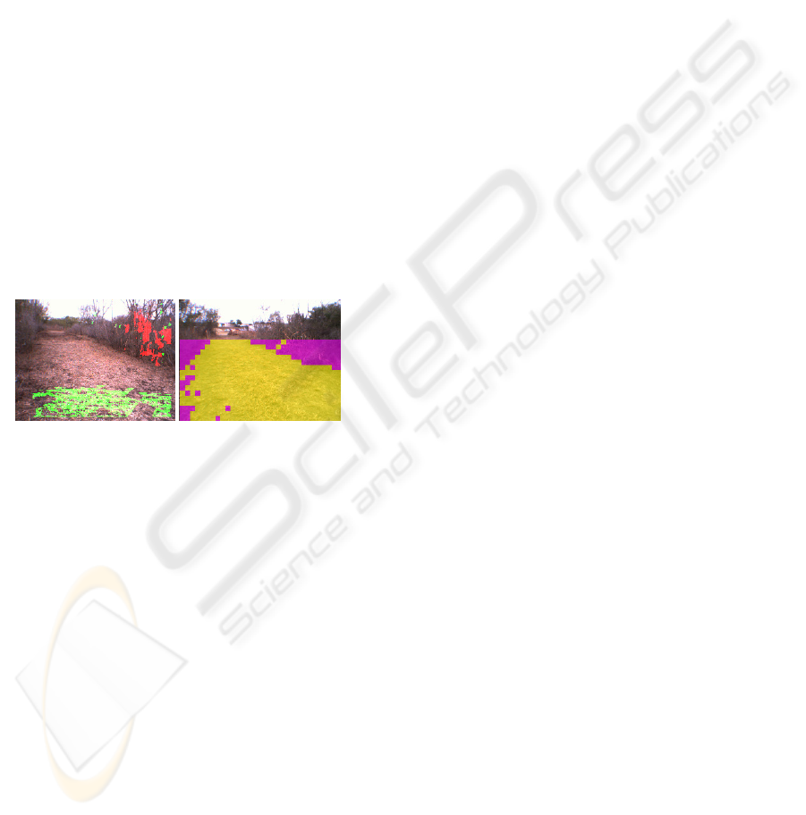
Figure 9a shows an image taken during learn-
ing. The pixels contributing to the learning are
shown in red for obstacle points and green for
ground points. Figure 9b shows a scene labeled with
traversability values computed from the models built
from previous data.
ICINCO 2006 - ROBOTICS AND AUTOMATION
160
4 SUMMARY AND
CONCLUSIONS
The NIST 4D/RCS reference model architecture was
implemented on the DARPA LAGR vehicle, which
was used to prove that 4D/RCS can learn. Sensor
processing, world modeling, and behavior genera-
tion processes have been described in this paper.
Outputs from sensor processing of vehicle sensors
are fused with models in WM to update them with
external vehicle information. World modeling acts as
a bridge between multiple sensory inputs and a be-
havior generation (path planning) subsystem. Behav-
ior generation plan vehicle paths through the world
based on cost maps provided from world modeling.
Learning, as used on the LAGR vehicle includes
learning by example, learning from experience, and
learning of behaviors that are more likely to lead to
success.
Future research will include completion of the
sensory processing upper level (SP2) and developing
even more robust control algorithms than those de-
scribed in this paper.
(a) (b)
Figure 9: Learning by example images. (a) is an image
taken during learning and overlaid with (red) obstacles
and (green) ground, (b) is the same image overlaid with
traversability information as obstacles (magenta) and
ground (yellow).
REFERENCES
Albus, J.S., Juberts, M., Szabo, S., RCS: A Reference
Model Architecture for Intelligent Vehicle and High-
way Systems, Proceedings of the 25th Silver Jubilee
International Symposium on Automotive Technology
and Automation, Florence, Italy, June 1-5, 1992.
Albus, J.S., Huang, H.M., Messina, E., Murphy, K.N.,
Juberts, M., Lacaze, A., Balakirsky, S.B., Shneier,
M.O., Hong, T.H., Scott, H.A., Proctor, F.M., Shackle-
ford, W., Michaloski, J.L., Wavering, A.J., Kramer,
Tom , Dagalakis, N.G., Rippey, W.G., Stouffer, K.A.,
4D/RCS Version 2.0: A Reference Model Architecture
for Unmanned Vehicle Systems, NISTIR, 2002.
Albus, J.S., Balakirsky, S.B., Messina, E., Architecting A
Simulation and Development Environment for Multi-
Robot Teams, Proceedings of the International Work-
shop on Multi Robot Systems, Washington, DC, March
18 – 20, 2002
Balakirsky, S.B., Chang, T., Hong, T.H., Messina, E.,
Shneier, M.O., A Hierarchical World Model for an
Autonomous Scout Vehicle, Proceedings of the SPIE
16th Annual International Symposium on Aero-
space/Defense Sensing, Simulation, and Controls, Or-
lando, FL, April 1-5, 2002.
Bostelman, R.V., Jacoff, A., Dagalakis, N.G., Albus, J.S.,
RCS-Based RoboCrane Integration, Proceedings of
the International Conference on Intelligent Systems: A
Semiotic Perspective, Gaithersburg, MD, October 20-
23, 1996.
Chang, T., Hong, T., Legowik, S., Abrams, M., Conceal-
ment and Obstacle Detection for Autonomous Driving,
Proceedings of the Robotics & Applications Confer-
ence, Santa Barbara, CA, October, 1999.
Heyes-Jones, J., A* algorithm tutorial, 2005
http://us.geocities.com/jheyesjones/astar.html.
Shneier, M., Chang, T., Hong, T., and Shackleford, W.,
Learning Traversability Models for Autonomous Mo-
bile Vehicles, Autonomous Robots (submitted), 2006.
Jackel, Larry, LAGR Mission,
http://www.darpa.mil/ipto/programs/lagr/index.htm,
DARPA Information Processing Technology Office,
2005
Konolige, K., SRI Stereo Engine, 2005
http://www.ai.sri.com/~konolige/svs/.
Michaloski, J.L., Warsaw, B.A., Robot Control System
Based on Forth, Robotics Engineering, Vol. 8, No. 5,
pgs 22-26, May, 1896.
Ojala, T., Pietikäinen, M., and Harwood, D., A Compara-
tive Study of Texture Measures with Classification
Based on Feature Distributions, Pattern Recognition,
29: 51-59, 1996.
Oskard, D., Hong, T., Shaffer, C., Real-time Algorithms
and Data Structures for Underwater Mapping, Na-
tional Institute of Standards and Technology, 1990.
Shackleford, W., The NML Programmer's Guide (C++
Version), 1990.
http://www.isd.mel.nist.gov/projects/rcslib/NMLcpp.ht
ml.
Shackleford, W., Stouffer, K.A., Implementation of
VRML/Java Web-based Animation and Communica-
tions for the Next Generation Inspection System
(NGIS) Real-time Controller, Proceedings of the
ASME International 20th Computers and Information
in Engineering (CIE) Conference, Baltimore, MD,
September 10 – 13, 2000.
Tan, C., Hong, T., Shneier, M., and Chang, T., "Color
Model-Based Real-Time Learning for Road Follow-
ing," in Proc. of the IEEE Intelligent Transportation
Systems Conference (Submitted) Toronto, Canada,
2006
THE LAGR PROJECT - Integrating Learning into the 4D/RCS Control Hierarchy
161
