COMBINING REINFORCEMENT LEARNING AND GENETIC

ALGORITHMS TO LEARN BEHAVIOURS IN MOBILE ROBOTICS

R. Iglesias

, M. Rodr

ıguez

, C.V. Regueiro

, J. Correa

and S. Barro

Electronics and Computer Science, University of Santiago de Compostela, Spain.

Dept. of Electronic and Systems, University of Coru˜na, Spain.

Keywords:

Robot Control, mobile robotics, autonomous agents, reinforcement learning, genetic algorithms.

Abstract:

Reinforcement learning is an extremely useful paradigm which is able to solve problems in those domains

where it is difﬁcult to get a set of examples of how the system should work. Nevertheless, there are important

problems associated with this paradigm which make the learning process more unstable and its convergence

slower. In our case, to overcome one of the main problems (exploration versus exploitation trade off), we

propose a combination of reinforcement learning with genetic algorithms, where both paradigms inﬂuence

each other in such a way that the drawbacks of each paradigm are balanced with the beneﬁts of the other.

The application of our proposal to solve a problem in mobile robotics shows its usefulness and high perfor-

mance, as it is able to ﬁnd a stable solution in a short period of time. The usefulness of our approach is

highlighted through the application of the system learnt through our proposal to control the real robot.

1 INTRODUCTION

Currently, there are three major learning paradigms in

artiﬁcial intelligence: supervised learning, unsuper-

vised learning, and reinforcement learning. By means

of reinforcement learning (RL), a system operating

in an environment learns how to perform a task in

that environment starting from a feedback called re-

inforcement which tells the system how good or bad

it has performed, but nothing about the desired re-

sponses. This is extremely useful in many domains,

such as mobile robotics, where it is quite difﬁcult or

even impossible to tell the system which action or de-

cision is the suitable one for every situation the system

might face.

To determine the desired behaviour the system

should attain after the learning procedure, it is just

necessary to deﬁne appropriately the reinforcement

function.

There are, however, certain difﬁculties associated

with the reinforcement learning methods. It is pos-

sible to mention, for example, the problems arising

from the fact that RL assumes that the environment as

perceived by the system is a Markov Decision Process

(MDP), which implies that the system only needs to

know the current state of the process in order to deter-

mine the suitable action to be carried out or to predict

its future behaviour. However, in many real situations

this is not hold.

During the learning process the action the system

should take at every state is determined. The set of

actions which solve the task maximizing the amount

of positive reinforcement the system receives is called

optimal policy. Usually RL demonstrates a slow con-

vergence to the optimal policy. Moreover, during the

search of this optimal policy the system encounters

a new and very important problem, brought about by

the fact that during the learning process new actions

for each of the possible states must be explored, in

order to verify which is the best action to take. Never-

theless, with the aim of maximising the reinforcement

received, the system would prefer to execute those ac-

tions that it has tried in the past and has found to be

effective in producing reward. As a consequence, the

system has to exploit what it already knows in order

to obtain a reward, but it also has to explore what it

does not know in order to make a better action selec-

tion in the future. This is what is called exploration

versus exploitation trade off.

The exploration versus exploitation trade off is one

of the main drawbacks of the reinforcement learning

paradigm, and it is also the main issue in this arti-

cle. The main disadvantages derived from this prob-

lem are, on one hand, the convergence time: the time

188

Iglesias R., Rodríguez M., V. Regueiro C., Correa J. and Barro S. (2006).

COMBINING REINFORCEMENT LEARNING AND GENETIC ALGORITHMS TO LEARN BEHAVIOURS IN MOBILE ROBOTICS.

In Proceedings of the Third International Conference on Informatics in Control, Automation and Robotics, pages 188-195

DOI: 10.5220/0001209501880195

 SciTePress

needed to learn a good policy increases exponentially

with the number of states the system might encounter

and the number of actions that it is possible to execute

in each one of them. On the other hand, the system

wastes too much time trying actions that are clearly

inappropriate for the task, but are selected randomly

in the exploration phase.

Exploration can be costly and impossible to carry

out in real systems where the execution of wrong ac-

tions might cause physical damage in the hardware.

Most of the work being done to speed up the learn-

ing process can be classiﬁed in one of two different

research options: a) The basic RL algorithms are be-

ing improved to increase the inﬂuence (in time) of the

wrong actions: if the system does something wrong

there is a high probability that the next time the sys-

tem visits the same or a similar sequence of states, it

tries something new. b) Some other mechanisms are

being developed to allow the injection of knowledge

or advice in the system.

In the work we describe in this paper, there is no

knowledge or advice injection in the learning phase.

We speed up the learning procedure through the com-

bination of RL and genetic algorithms. Our aim is

to propose a mechanism where the exploration is fo-

cused thus decreasing the learning time, and increas-

ing the stability of the learning process.

The structure of the article is divided in the follow-

ing sections: First, we will describe brieﬂy the basic

principles of reinforcement learning (section 2). The

basic aspects of genetic algorithms and how they are

combined with reinforcement learning is described in

section 3. Section 4 presents the application of the

proposal described in this article to solve a problem

in the mobile robotics domain. Finally, the conclu-

sion and future research are summarized in section 5.

2 REINFORCEMENT LEARNING

ALGORITHMS

This section includes some basic aspects regarding re-

inforcement learning (RL), and more speciﬁcally on

one of its algorithms, known as truncated temporal

differences TTD(λ, m) (Cichosz, 1997).

We will assume that a system interacts with the en-

vironment at discrete time steps. The environment

must be at least partially observable by the system, in

such a way that it is able to translate the different situ-

ations that it may detect into a ﬁnite number of states,

S. At each step, the system observes the current state,

s(t) ∈ S, and performs an action a(t) ∈ A, where A

is the ﬁnite set of all possible actions. The immediate

effect of the execution of an action is a state transi-

tion, and scalar reinforcement value, which tells the

system how good or badly it has performed.

TTD(λ, m) algorithm learns a utility function of

states and actions called the Q-function. Thus, for

the current state s

, Q

, a) is the total discounted

reinforcement that will be received starting from state

, executing action a, and then following policy π,

(where a policy is a function that associates a particu-

lar action a ∈ A for each state s ∈ S ).

, a) =

∞

k=0

t+k

, γ ≤ 1

In order to learn this utility function, the system

starts with a randomly chosen set of negative values

Q(s, a), ∀s, a and then initiates a stocastical explo-

ration of its environment. As the system explores, it

continually makes predictions about the reward it ex-

pects, and then it updates its utility function by com-

paring the reward it actually receives with its predic-

tion. Thus, the TTD(λ, m) algorithm could be sum-

marized through the following steps:

At each instant, t:

1. Observe the current state, s(t): s[0] = s(t).

2. Select an action a(t) for s(t): a[0] = a(t).

3. Perform action a(t), observe new state s(t+1) and

reinforcement value r(t).

4. r[0] = r(t), u[0] = max

(s(t + 1), a)

5. for k = 0, 1, . . . , m − 1 do:

• if k = 0 then z = r[k] + γu[k]

• else z = r[k] + γ(λz + (1 − λ)u[k]), where

0 < γ, λ ≤ 1.

6. Update the Q-values:

• ∆ = z − u[s[m − 1])

• Q

t+1

(s[m−1], a[m−1]) = Q

(s[m−1], a[m−

1]) + β∆

7. Shift the indexes of the experience buffer.

It is important to notice the system keeps track of

the ”m” most recent states. The consequences of ex-

ecuting action a at time t, are backpropagated m − 1

steps earlier.

The optimal policy which maximizes the amount

of reinforcement the system receives is called greedy

policy, π

∗

. This policy establishes that the action to

be carried out at every state, s ∈ S, is the one which

seems to be the best one according to the Q-values:

∗

(s) = argmax

Q(s, a)

The greedy policy determines the behaviour of the

system after the learning process.

2.1 Action Selection Mechanism

In order to determine the action to be executed at

every instant (step 2 in the T T D(λ, m) algorithm),

COMBINING REINFORCEMENT LEARNING AND GENETIC ALGORITHMS TO LEARN BEHAVIOURS IN

MOBILE ROBOTICS

189

there are many options. Basically all of them try to

keep a high exploration ratio at the beginning of the

learning procedure while, as time goes by, more and

more the selected actions are those which are consid-

ered the best (according to the Q-values).

A good example is the exploration based on the

Boltzman distribution. According to this strategy, the

probability of executing action a

∗

in state s(t), is

given by the following expression:

P rob(s(t), a

∗

) =

Q(s(t),a

∗

)/T

∀a

Q(s(t),a)/T

, (1)

where the value T > 0 is a temperature that controls

the randomness. Very low temperatures cause nearly

deterministic action selection, while high values re-

sult in random performances.

3 COMBINING GENETIC

ALGORITHMS WITH

REINFORCEMENT

LEARNING: GA+RL

A genetic algorithm (GA) is a biologically inspired

search technique very suitable to ﬁnd approximate

solutions to optimization search problems (Davidor,

1991). This algorithm is based on the evolutionary

ideas of natural selection and genetic. In general ge-

netic algorithms are considered to be useful when the

search space is large, complex or poorly understood,

the domain knowledge is scarce or expert knowledge

is difﬁcult to encode, and a mathematical analysis of

the problem is difﬁcult to carry out.

To solve a search problem the GA begins with a

population of solutions (called chromosomes). Each

chromosome of this population is evaluated using

an objective function, called ﬁtness function, which

measures how close is the chromosome to the desired

solution. A new population is then obtained from the

ﬁrst one, according to the ﬁtness values: the better a

chromosome seems to be, the higher the probability

that chromosome is selected for the new population

of solutions. To keep certain randomness in the al-

gorithm, which prevents it from being trapped in a lo-

cal minimum, the application of genetic operators like

chromosome mutation (random changes in the pro-

posed solution), or chromosome crossover (combina-

tion of two chromosomes to raise two new solutions),

is required when a new set of solutions is obtained

from a previous one.

The evaluation of the population of solutions, and

its evolution to a new and improved population, are

two steps which are repeated continuously until the

desired behaviour is reached.

In our case we wanted to combine the potential of

a GA with RL (ﬁgure 1), in such a way that the draw-

backs of each paradigm are balanced with the beneﬁts

of the other.

3.1 How a GA Improves RL

Genetic algorithms help RL in generalization and se-

lectivity (David E. Moriarty, 1999). GA learns a map-

ping from observed states to recommended actions,

usually eliminating explicit information concerning

less desirable actions. In a GA the knowledge about

bad decisions is not explicitly preserved, since poli-

cies that make such decisions are not selected by the

evolutionary algorithm and are eventually eliminated

from the population. Thus, because the attention is

only focused on proﬁtable actions and less informa-

tion has to be learnt, the system reaches globally good

solutions faster than RL.

As can be seen through ﬁgure 1, RL and GA share

the same ﬁnite number of states, S, which represent

the different situations the system may detect. Thus,

a chromosome and a policy are both the same, as a

chromosome also has to establish the action a ∈ A,

to be carried out at every state s ∈ S (this coincides

with the deﬁnition of policy given in section 2). Ac-

cording to ﬁgure 1, the ﬁtness is a function of the re-

ward values. The longer a chromosome/policy is able

to control the system properly, the higher its ﬁtness

value is.

When a set of N policies are being evaluated, if one

of them makes the system behave much better than

the others, there is a big probability that similar se-

quences of actions are explored through the next gen-

erated population of chromosomes. In RL, this is not

possible, as it would require a high learning coefﬁ-

cient and a fast decrease of the temperature coefﬁcient

(towards the greedy policy). This high learning coef-

ﬁcient would cause important instabilities during the

learning process, as the execution of correct actions

in the middle of wrong ones, would quickly decrease

their Q-values.

3.2 How RL Improves GA

As pointed out previously RL keeps more informa-

tion than GA. The Q-values reﬂect the consequences

of executing every possible action in each state. This

information might be useful to bias the genetic opera-

tors to reduce the number of chromosomes required to

ﬁnd a solution. Thus, the mutation probability could

be higher for those policies and states where the se-

lected action is poor according to the Q-values, the

crossover between two policies could be in such a way

that the exchanged actions have similar Q-value, etc.

In our proposal, the ﬁrst genetic operator which

saw its way of functioning changed was the mutation

ICINCO 2006 - ROBOTICS AND AUTOMATION

190

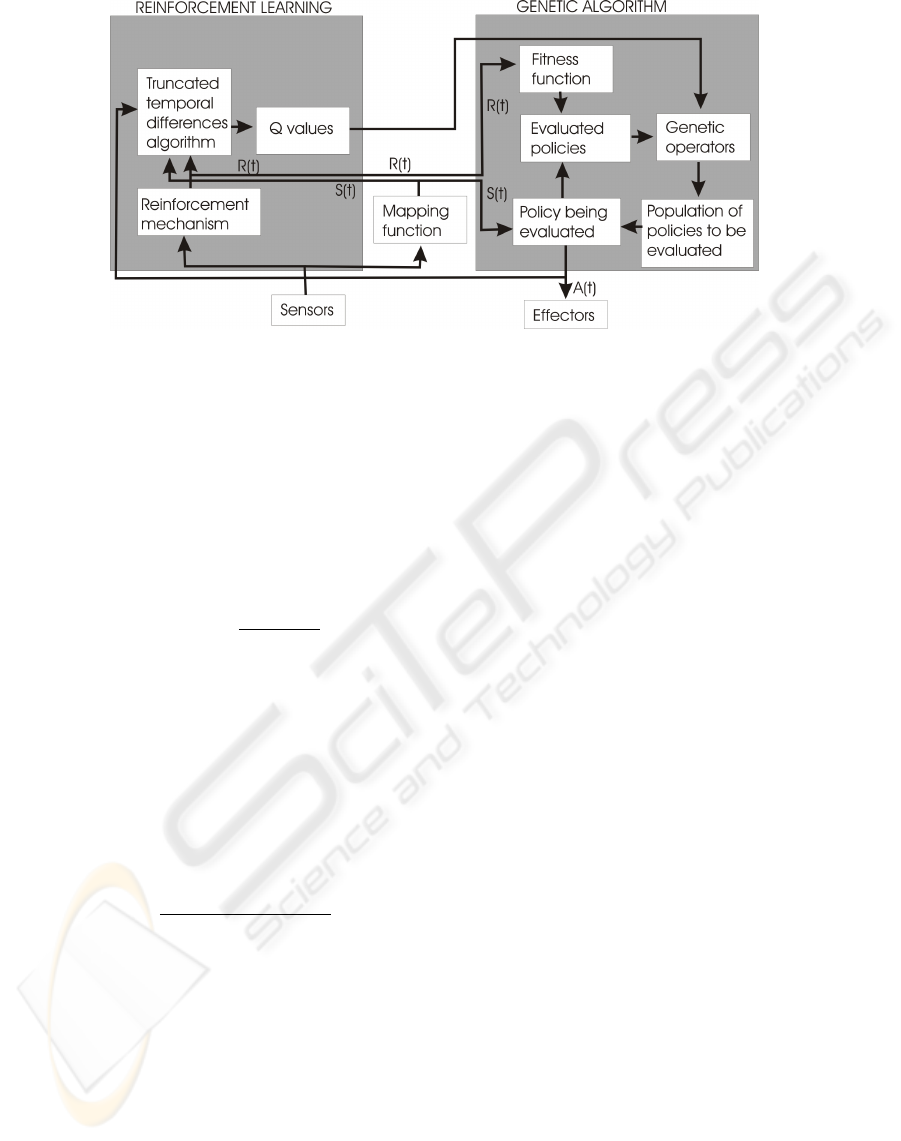
Figure 1: Representation of our proposal to combine GA with RL.

operator. For each chromosome, π, the probability

that mutation changes the action that it suggests for a

particular state, π(s), depends on how many actions

look better or worse -according to the Q-values- than

the one suggested by the chromosome:

N1 = cardinality{a

| Q(s, a

) ≥ Q(s, π(s))}

N2 = cardinality{a

| Q(s, a

) ≤ Q(s, π(s))}

mutation

(π(s)) =

N1 + N2

N1 represents the number of actions that look bet-

ter than π(s), N2 the number of worse actions than

π(s). P

mutation

(π(s)) establishes the probability that

mutation changes the action suggested by policy π

in state s. Nevertheless, if mutation is going to be

carried out, there is a big uncertainty about which

other action, instead of π(s), should be selected. In

our case, instead of a random selection, there is a

probability of picking up every action, P

(s, a

), ∀a

which depends on the Q-values:

(s, a

) =

Q(s,π (s )) /Q(s,a

)

Q(s,π (s )) /Q(s,a

)

. (2)

Those actions whose Q-values are higher than the one

corresponding to the action currently proposed, have

a higher probability of being selected as new can-

didates than those other actions whose Q-values are

lower than the one corresponding to π(s).

To understand equation 2, it is important to bear in

mind that Q(s, a

) ≤ 0, ∀a

3.2.1 Non Episodic Tasks

An episodic task is one in which the agent-

environment interaction is divided into a sequence of

trials, or episodes. Each episode starts in the same

state, or in a state chosen from the same distribution,

and ends when the environment reaches a terminal

state. A continuous task is the opposite of an episodic

one, there is one episode that starts once and goes for-

ever. There are situations where a continuous task can

be also broken into different episodic subtasks.

When the task is continuous there might be prob-

lems evaluating and comparing different policies us-

ing Genetic Algorithms, as the starting position of the

system is not always the same. On the other hand,

in the case of a continuous task which is broken into

episodic subtasks, the population of policies might

evolve to solve a subtask, but once that subtask is

solved, the population might be useless for the next

subtask. Moreover, if the set of all possible environ-

mental states is the same for all the subtasks, it could

happen that the policies evolve to solve a subtask but

they forget how to solve all the previous ones.

To be able to work just with a population of chro-

mosomes, even when dealing with a continuous task,

one of the chromosomes of the population must al-

ways be the greedy policy obtained from the Q-

values. The reason is that the Q-values group together

all the experiences the system has gone through. In

this sense, the RL algorithm helps GA to have a fast

convergence to the desired solution.

3.2.2 Non-Stationary Environments

As it is described in (David E. Moriarty, 1999), when

the agent’s environment changes over time, the RL

problem becomes even more difﬁcult, since the op-

timal policy becomes a moving target. To increase

the performance of a GA to rapidly changing environ-

ments, it would be necessary a higher mutation rate

(Cobb and Grefenstette, 1993), or keep a randomized

portion of the population of chromosomes (Grefen-

stette, 1992).

COMBINING REINFORCEMENT LEARNING AND GENETIC ALGORITHMS TO LEARN BEHAVIOURS IN

MOBILE ROBOTICS

191

3.3 Main Stages in the Learning

Process

When our GA+RL approach is used there are three

basic stages which are repeated cyclically during

the learning process: a) Evaluation: the chromo-

somes/policies are evaluated when the system starts

always from the same position in the environment.

During this stage the Q-values are updated. b) New

population generation: Using the genetic operators

biased with the Q-values, a new population of policies

is generated. c) Checking for a new starting position

or convergence: The greedy policy is used to control

the system. If it does something wrong, the position

of the system several steps before the failure is estab-

lished as a new starting position for the next evalu-

ation stage. If the greedy policy is able to properly

control the system for a signiﬁcant interval of time,

convergence is detected and the learning procedure is

stopped.

4 APPLICATION OF GA-RL TO

MOBILE ROBOTICS

We applied both, the reinforcement learning algo-

rithm T T D(λ, m) and the GA+RL mechanism, to

learn robot controllers which are able to solve a com-

mon task in mobile robots: ”wall following”. The

controllers must determine the commands the robot

should carry out to follow a wall located on its right

and at certain distance interval, using only the in-

formation provided by the right side sensors. Our

aim here is not to achieve the best wall following

behaviour, but to show how our proposal is able to

solve the problem applying a learning process which

is faster that the one corresponding to RL.

The robot we used is a Nomad200 robot equipped

with 16 ultrasound sensors encircling its upper part,

16 infrared sensors, laser and bumpers.

The ﬁnite set of states through which the environ-

ment around the robot is identiﬁed is the same regard-

less of the learning paradigm we used. Because of

this, we’ll describe ﬁrst how we obtained this state

representation, and then we’ll describe the results ob-

tained when T T D(λ, m) and GA+RL were used.

4.1 Representation of the

Information: Obtaining the State

of the Environment

To translate the large number of different situations

that the ultrasound sensors may detect into a ﬁnite

and reduced set of environmental identiﬁcation states,

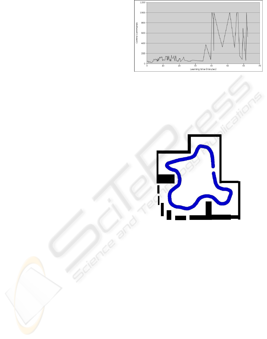
Figure 2: Maxim um number of commands that the greedy

policies, saved during the learning stage, are able to send to

the robot before it does something wrong in either of the

two environments: the training or the testing one. 1000

commands is the maximum number of commands any pol-

icy can send to the robot before being considered as correct

and its evaluation ﬁnished. T T D(λ, m) was applied.

Figure 3: Robot’s trajectory in the training environment.

40 minutes and 20 seconds were necessary to learn the

control policy which determines the robot’s movement.

T T D(λ, m) was used.

a set of layered Kohonen networks was used (R. Igle-

sias and Barro, 1998a). In the ﬁrst layer we have em-

ployed 5 one dimensional Kohonen networks with 15

neurones each. The inputs of each one-dimensional

network are the readings from three adjacent sensors.

The output of these networks is a ﬁve component vec-

tor which codiﬁes and abstracts the environment visi-

ble through the robot’s right ultrasound sensors. Nev-

ertheless, it is clearly not viable to associate each one

of these vectors to a state, as this would mean han-

dling with 15

states. The necessary reduction in the

number of ﬁnal states has been achieved by means

of a hexagonal bidimensional Kohonen network of

22 × 10 neurones. Thus, at every instant, the envi-

ronment surrounding the robot is identiﬁed through

one of these 220 neurones.

ICINCO 2006 - ROBOTICS AND AUTOMATION

192

4.2 Application of the Reinforcement

Learning Algorithm, T T D(λ, m),

to Learn the Robot Controller

We ﬁrst learnt the robot controller using the

T T D(λ, m) learning algorithm described in section

2. The linear velocity of the robot is kept constant

in all the experiments (15.24 cm/s). To determine

the most suitable values of the learning parameters

we analysed the time required to learn the task when

they were changed. In particular we tried with β =

{0.25, 0.35, 0.45, 0.55}, λ = {0.4, 0.5, 0.60.7, 0.8},

and m = {10, 20, 30, 40, 50}. The best combina-

tion of parameters we found is β = 0.35, λ = 0.8,

γ = 0.95 and m = 30. The reinforcement learning

function penalizes those situations where the robot

is too close or too far from the wall being followed

(r = −2), being r = 0 otherwise.

Finally, to determine the action the robot should

carry out at every instant, t, an exploration strategy

based on the Bolztman distribution was used (equa-

tion 1). According to this strategy, the probability of

selecting action a, in the current state s(t), depends

on the Q-value, Q(s(t), a), and a decreasing temper-

ature T > 0. In our case, as there is a signiﬁcant

difference in the relative frequency of the 220 possi-

ble states, we worked with a temperature value which

is independent for each of them: T (s). Each time the

robot is faced with a particular state s(t) , the tem-

perature of this state s(t) is reduced with a constant

ratio:

t+1

(s(t)) = 0.999T (s(t))

The decreasing ratio of the temperature has been se-

lected in such a way that after 9206 times visiting the

same state, there is a high probability that the action

selected to execute in that state is always the best one

according to the Q-values.

Finally, because we want to compare the movement

of the robot when different controllers are used, the

robot receives a command with the action to be car-

ried out every 300 ms.

In order to learn the task, the behaviour of the robot

was simulated in a training environment, and tested

in a different one, ﬁgures 3 and 4. The greedy poli-

cies at different instants of time were saved during

the learning process, with the purpose of evaluating

each one of them afterwards, ﬁgure 2. In particu-

lar it is determined how many commands each policy

is able to send to the robot before it does something

wrong whereas if the robot doesn’t fail at all during

1000 commands (5 minutes of movement), the policy

is taken as correct and its evaluation is then ﬁnished.

According to ﬁgure 2, around 42 minutes are

roughly enough to learn the desired task. The problem

is that as we can see in the graph, the convergence is

not very stable –the greedy policy learnt by the robot

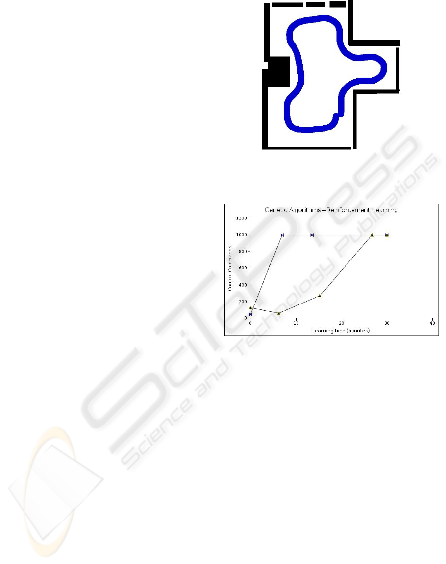
Figure 4: Robot’s trajectory in the testing environment

when the same control policy as the one applied in ﬁgure

3 is used.

Figure 5: Maxim um number of commands that the greedy

policies saved during two different learning processes are

able to send to the robot. After 1000 commands the policy

is considered correct and its evaluation ﬁnished. GA+RL

was applied.

after convergence is occasionally wrong–. As we can

see in the trajectory shown in ﬁgure 4, the controller is

able to solve the task, although there are parts where

the robot is too far from the wall being followed.

The best values we found for the parameters

present in the RL algorithm have been used in all the

experiments we carried out (using RL or GA+RL).

4.3 Application of GA+RL to Learn

the Robot Controller

Our GA+RL proposal has proved to be much faster

than the T T D(λ, m) algorithm (ﬁgure 5). We re-

peated the experiment 4 times and the average time

required to learn the behaviour was 24.27 minutes.

There are 20 policies (chromosomes) being evaluated

and evolved, 6 of them are random policies (to face

with non-static environments and keep a suitable ratio

COMBINING REINFORCEMENT LEARNING AND GENETIC ALGORITHMS TO LEARN BEHAVIOURS IN

MOBILE ROBOTICS

193

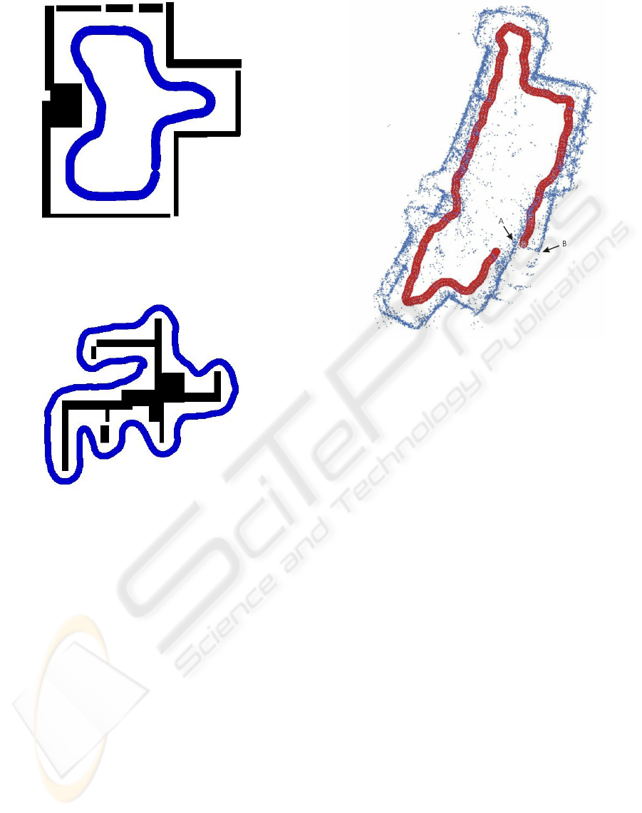
Figure 6: Robot’s trajectory in the testing environment

when a control policy which has been learnt in 27 minutes

and 45 seconds is used. GA+RL was applied.

Figure 7: Robot’s trajectory in a new and complex envi-

ronment using a control policy learnt through the use of

GA+RL.

of exploration), and one of the remaining ones is the

greedy policy (because this is a non-episodic task).

Through the experiments we carried out, we have no-

ticed that increasing the total number of policies being

evaluated doesn’t help to have a faster convergence.

We also could see that the most suitable number of

random policies is 30% of the whole population.

Regarding the three basic stages described in sec-

tion 3.3 that are repeated cyclically: a) Evaluation,

b) New population generation, and c) Checking for a

new starting position or convergence, it is necessary

to specify here that in the third stage the greedy pol-

icy is used to control the robot. If it does something

wrong, the position of the robot several steps before

the failure is established as a new starting position for

the next evaluation stage. If the greedy policy is able

to properly control the movement of the robot for an

interval of 15 minutes, convergence is detected and

the learning procedure is stopped.

Through ﬁgures 6 and 7, we can see how GA+RL

Figure 8: Real robot’s trajectory in a noisy and real envi-

ronment when the same control policy as the one showed in

ﬁgure 7 is used to control the robot’s movement. Points A

and B in the graph are the same, the misalignment is due to

the odometry error. The small dots in the graph correspond

to the ultrasound readings.

can be used to learn controllers which are able to

move the robot in two very different and complex en-

vironments. Moreover, to prove that the behaviours

learnt with the GA+RL proposal are useful, ﬁgure 8

shows the movement of the real robot in a real and

noisy environment when one of the greedy policies

learnt with GA+RL is used to control it.

In this article we also claim that through the combi-

nation of GA and RL the stability of the learning pro-

cess is increased. Figure 9 conﬁrms this, as it shows

how the number of negative reinforcements received

during the learning stage is lower with GA+RL (1444)

than with T T D(λ, m) (4799).

5 CONCLUSIONS AND FUTURE

WORK

Reinforcement learning is an extremely useful

paradigm where the speciﬁcation of the restrictions

of the aimed behaviour of the system is enough to

start a random search of the desired solution. Nev-

ertheless, a successful application of this paradigm

requires a good exploration strategy, suitable to ﬁnd

a good solution without a deep search through all the

possible combinations of actions, which might desta-

ICINCO 2006 - ROBOTICS AND AUTOMATION

194

Figure 9: Number of negative reinforcements received dur-

ing the learning stage when different strategies are used.

bilize the system and increase enormously the conver-

gence time.

In our case, we proposed the combination of ge-

netic algorithms and reinforcement learning, in such

a way that the mutual inﬂuence of both paradigms

strength their potential and correct their drawbacks.

Through our proposal, the exploration strategy is im-

proved and the time required to ﬁnd the pursuit solu-

tion is reduced drastically.

Our ﬁrst experimental results after the application

of our proposal to solve a particular problem in mo-

bile robotics, conﬁrm that there are situations where

our approach is viable and its performance really

high. The changes necessary to carry out in order to

join our proposal with a dynamic generation of the

states which identify the environment around the sys-

tem (R. Iglesias and Barro, ), or the injection of prior

knowledge of the task (R. Iglesias and Barro, 1998b),

is subject to ongoing research.

ACKNOWLEDGEMENTS

The authors thank the support received through the

research grants PGIDIT04TIC206011PR, TIC2003-

09400-C04-03 and TIN2005-03844.

REFERENCES

Cichosz, P. (1997). Reinforcement Learning by Truncating

Temporal Differences. PhD thesis, Dpt. of Electron-

ics and Information Technology, Warsaw University

of Technology.

Cobb, H. G. and Grefenstette, J. J. (1993). Genetic al-

gorithms for tracking changing environments. In

Proc. Fifth International Conference on Genetic Al-

gorithms.

David E. Moriarty, Alan C. Schultz, J. J. G. (1999). Evolu-

tionary algorithms for reinforcement learning. Journal

of Artiﬁcial Intelligence Research, 11:241–276.

Davidor, Y. (1991). Genetic algorithms and robotics. A

heuristic strategy for optimization. World Scientiﬁc.

Grefenstette, J. J. (1992). Parallel Problem Solving from

Nature, volume 2, chapter Genetic algorithms for

changing environments.

R. Iglesias, C. V. Regueiro, J. C. and Barro, S. (1998a). Im-

proving wall following behaviour in a mobile robot

using reinforcement learning. In ICSC International

Symposium on Engineering of Intelligent Systems,

EIS’98.

R. Iglesias, C. V. Regueiro, J. C. and Barro, S. (1998b).

Supervised reinforcement learning: Application to a

wall following behaviour in mobile robotics. In Inter-

national Conference on Ingustrial & Engineering Ap-

plications of Artiﬁcial Intelligence & Expert Systems.

R. Iglesias, M. F. D. and Barro, S. Learning of perceptual

states in the design of an adaptive wall-following be-

haviour. In European Symposium on Artiﬁcial Neural

Networks, ESANN 2000.

COMBINING REINFORCEMENT LEARNING AND GENETIC ALGORITHMS TO LEARN BEHAVIOURS IN

MOBILE ROBOTICS

195