
VISUAL TOPOLOGICAL MAP BUILDING IN SELF-SIMILAR
ENVIRONMENTS
Toon Goedem
´
e, Tinne Tuytelaars and Luc Van Gool
PSI - VISICS
Katholieke Universiteit Leuven, Belgium
Keywords:
Mobile robot navigation, Topological map building, Omnidirectional vision, Dempster-Shafer theory.
Abstract:
This paper describes a method to automatically build topological maps for robot navigation out of a sequence
of visual observations taken from a camera mounted on the robot. This direct non-metrical approach relies
completely on the detection of loop closings, i.e. repeated visitations of one particular place. In natural
environments, visual loop closing can be very hard, for two reasons. Firstly, the environment at one place can
look differently at different time instances due to illumination changes and viewpoint differences. Secondly,
there can be different places that look alike, i.e. the environment is self-similar. Here we propose a method
that combines state-of-the-art visual comparison techniques and evidence collection based on Dempster-Shafer
probability theory to tackle this problem.
1 INTRODUCTION AND
RELATED WORK
In every mobile robot application, the internal repre-
sentation of the perceived environment is of crucial
importance. The environment map is the basis for
other tasks, like localisation, path planning, naviga-
tion, etc ...The map building field can be divided in
two major paradigms: geometrical maps and topo-
logical maps, even if hybrid types have been imple-
mented (Tomatis et al., 2002).
In the traditional geometrical paradigm, maps
are quantitative representations of the environment
wherein locations are given in metrical coordinates.
One approach often used is the occupancy map: a grid
of evenly spaced cells each containing the information
whether the corresponding position in the real world
is occupied.
Because the latter is error-prone, time-consuming,
and memory-demanding, we chose for the topological
paradigm. Here, the environment map is a qualita-
tive graph-structured representation where nodes rep-
resent distinct places in the environment, and arcs de-
note traversable paths between them. This flexible
representation is not dependent on metrical localisa-
tion such as dead reckoning, is compact, allows high-
level symbolic reasoning and mimics the internal map
humans and animals use (Tolman, 1948).
Several approaches for automatic topological map
building have been proposed, differing in the method
and the sensor(s) used. In our work, we solely use a
camera as sensor. We chose for an omnidirectional
system with a wide field-of-view.
Other researchers worked mainly with other sen-
sors, such as the popular laser range scanner. A stan-
dard approach is the one of (Nagatani et al., 1998),
who construct generalised Voronoi diagrams out of
laser range data.
Very popular are various probabilistic approaches
of the topological map building problem. (Ran-
ganathan et al., 2005) for instance use Bayesian in-
ference to find the topological structure that explains
best a set of panoramic observations, while (Shatkay
and Kaelbling, 1997) fit hidden Markov models to
the data. If the state transition model of this HMM
is extended with robot action data, the latter can be
modeled using a partially observable Markov deci-
sion process or POMDP, as in (Koenig and Simmons,
1996) and (Tapus and Siegwart, 2005). (Zivkovic
et al., 2005) solve the map building problem using
graph cuts.
In contrast to these global topology fitting ap-
proaches, an alternative way is detecting loop clos-
ings. During a ride through the environment, sensor
data is recorded. Because it is known that the driven
path is traversable, an initial topological representa-
tion is one long edge between start and end node.
Now, extra links are created where a certain place
is revisited, i.e. an equivalent sensor reading occurs
3
Goedemé T., Tuytelaars T. and Van Gool L. (2006).
VISUAL TOPOLOGICAL MAP BUILDING IN SELF-SIMILAR ENVIRONMENTS.
In Proceedings of the Third International Conference on Informatics in Control, Automation and Robotics, pages 3-9
DOI: 10.5220/0001209200030009
Copyright
c
SciTePress

twice in the sequence. This is called a loop closing.
A correct topological map results if all loop closing
links are added.
In natural environments, loop closing based on
mere vision input can be very hard, for two rea-
sons. Firstly, the environment at one place can look
different at different time instances due to illumina-
tion changes, viewpoint differences and occlusions.
A comparison technique that is not robust to these
changes will overlook some loop closings. Secondly,
there can be different places that look alike, i.e. the
environment is self-similar. These would add erro-
neous loop closings and thus yield an incorrect topo-
logical map as well.
In (Wahlgren and Duckett, 2005), the authors de-
tect loops by comparing omnidirectional images with
local feature techniques, a robust technique we also
adopt. But, there method suffers indeed from self-
similarities, as we experienced in previous work
(Goedem
´
e et al., 2004b).
Also in loop closing, probabilistic methods are in-
troduced to cope with the uncertainty of link hy-
potheses. (Chen and Wang, 2005), for instance, use
Bayesian inference. (Beevers and Huang, 2005) re-
cently introduced Dempster-Shafer probability the-
ory into loop closing, which has the advantage that
ignorance can be modeled and no prior knowledge
is needed. Their approach is promising, but limited
to simple sensors and environments. In this paper,
we present a new framework for loop closing using
rich visual sensors in natural complex environments,
which is also based on Dempster-Shafer mathematics
but uses it differently.
We continue the paper with a brief summary of
Dempster-Shafer theory in section 2. Then we de-
scribe the details of our algorithm in section 3. Sec-
tion 4 details our real-world experiments. The paper
ends with a conclusion in section 5.
2 DEMPSTER-SHAFER
The proposed visual loop closing algorithm relies
on Dempster-Shafer theory (Dempster, 1967; Shafer,
1976) to collect evidence for each loop closing hy-
pothesis. Therefore, a brief overview of the central
concepts of Dempster-Shafer theory is presented in
this section.
Dempster-Shafer theory offers an alternative to tra-
ditional probabilistic theory for the mathematical rep-
resentation of uncertainty. The significant innova-
tion of this framework is that it makes a distinction
between multiple types of uncertainty. Unlike tra-
ditional probability theory, Dempster-Shafer defines
two types of uncertainty:
- Aleatory Uncertainty – the type of uncertainty
which results from the fact that a system can be-
have in random ways (a.k.a. stochastic or objective
uncertainty)
- Epistemic Uncertainty – the type of uncertainty
which results from the lack of knowledge about a
system (a.k.a. subjective uncertainty or ignorance)
This makes it a powerful technique to combine several
sources of evidence to try to prove a certain hypothe-
sis, where each of these sources can have a different
amount of knowledge (ignorance) about the hypothe-
sis. That is why Dempster-Shafer is typically used for
sensor fusion.
For a certain problem, the set of mutually exclu-
sive possibilities, called the frame of discernment, is
denoted by Θ. For instance, for a single hypothe-
sis H about an event this becomes Θ = {H, ¬H}.
For this set, traditional probability theory will define
two probabilities P (H) and P (¬H), with P (H) +
P (¬H) = 1. Dempster-Shafer’s analogous quantities
are called basic probability assignments or masses,
which are defined on the power set of Θ: 2
Θ
=
{A|A ⊆ Θ}. The mass m : 2
Θ
→ [0, 1] is a function
meeting the following conditions:
m(∅) = 0
X
A∈2
Θ
m(A) = 1. (1)
For the example of the single hypothesis H, the power
set becomes 2
Θ
= {∅, {H}, {¬H}, {H, ¬H}}. A
certain sensor or other information source can assign
masses to each of the elements of 2
Θ
. Because some
sensors do not have knowledge about the event (e.g.
it is out of the sensor’s field-of-view), they can assign
a certain fraction of their total mass to m({H, ¬H}).
This mass, called the ignorance, can be interpreted as
the probability mass assigned to the outcome ‘H OR
¬H’, i.e. when the sensor does not know about the
event, or is—to a certain degree—uncertain about the
outcome
1
.
Sets of masses about the same power set, coming
from different information sources can be combined
together using Dempster’s rule of combination:
m
1
⊕ m
2
(C) =
P
A∩B=C
m
1
(A)m
2
(B)
1 −
P
A∩B=∅
m
1
(A)m
2
(B)
(2)
This combination rule is useful to combine evidence
coming from different sources into one set of masses.
Because these masses can not be interpreted as classi-
cal probabilities, no conclusions about the hypothesis
can be drawn from them directly. That is why two ad-
ditional notions are defined, support and plausibility.
They are computed as:
Spt(A) =
X
B⊆A
m(B) P ls(A) =
X
A∩B6=∅
m(B)
(3)
1
This means also that no prior probability function is
needed, no knowledge can be expressed as total ignorance.
ICINCO 2006 - ROBOTICS AND AUTOMATION
4
These values define a confidence interval for
the real probability of an outcome: P (A) ∈
[Spt(A), P ls(A)]. Indeed, due to the vagueness im-
plied in having non-zero ignorance, the exact prob-
ability can not be computed. But, decisions can be
made based on the lower and upper bounds of this
confidence interval.
3 ALGORITHM
We apply this mathematical theory on loop closing
detection based on omnidirectional image input. Our
target application is as follows. A robot is equipped
with an omnidirectional camera system and is guided
through an environment, e.g. by means of a joystick.
While driving around, images are captured at con-
stant time intervals. This yields a sequence of images
which the automatic method described in this paper
transforms in a topological map. Later, this map can
be used for localisation, path planning and navigation,
as we described in previous work (Goedem
´
e et al.,
2004a) and (Goedem
´
e et al., 2005).
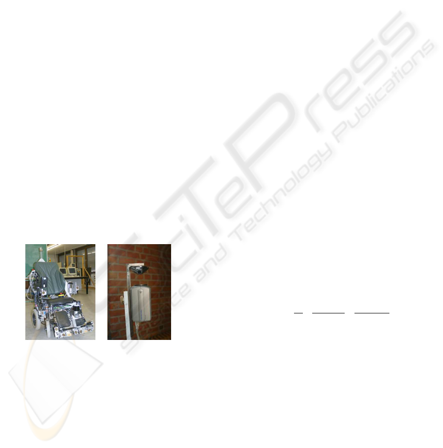
3.1 Omnidirectional Camera System
The visual sensor we use is a catadioptric system
composed by a colour camera and an hyperbolic mir-
ror, as shown in fig. 1. This system is mounted on top
of a robot, in our case the electric wheel chair Shari-
oto. Typical images are shown in fig. 7.
Figure 1: Left: the wheel chair test platform. Right: the
omnidirectional camera system.
3.2 Image Comparison
Because we do not have any other kind of informa-
tion, the entire topological loop closing is based on
images. The target is to find a good way to com-
pare images, such that a second visit to a certain place
can be detected as two similar images in the input se-
quence. As explained before, one of the main chal-
lenges is the appearance variation of places. At dif-
ferent time instances (i.e. during different visits), the
images acquired at a certain place can vary a lot. This
is mostly due to three reasons:
- Illumination differences: The same place is illu-
minated with a different light source (e.g. some-
body switched on a light, the sun emerges from be-
hind the clouds, .. .).
- Occlusions: Part of the image can be hidden be-
cause of e.g. people passing by.
- Viewpoint differences: It can never be guaranteed
that the robot comes back to exactly the same posi-
tion. Even for small viewpoint changes the image
looks different.
We want to recognise a place despite these factors,
requiring the image comparison to be invariant or at
least robust against them. Our proposed image com-
parison technique makes use of fast wide baseline fea-
tures, namely SIFT (Lowe, 2004) and Vertical Col-
umn Segments (Goedem
´
e et al., 2004c). These tech-
niques compute local feature matches between the
two images, invariant to the illumination. Such a local
technique is also robust to occlusions. Fig. 2 shows
an example of the found correspondences using these
two kinds of features. These matches were found in
less than half a second on up-to-date hardware and
640×480 images.
The required image comparison measure (visual
distance) must be inverse proportional to the number
of matches, relative to the average number of features
found in the images. Hence the first two factors in
equation 4. But, also the difference in relative con-
figuration of the matches must be taken in account.
Therefore, we first compute a global angular align-
ment of the images by computing the average angle
difference of the matches. The visual distance is now
also made proportional to the average angle difference
of the features after this global alignment.
d
V
=
1
N
·
n
1
+ n
2
2
·
P
|∆α
i
|
N
(4)
where N corresponds to the number of matches
found, n
i
the number of extracted features in image
i, ∆α
i
the angle difference for one match after global
alignment.
3.3 Image Clustering
We define a topological map as a graph; a set of
places is connected by links denoting possible tran-
sitions from one place to another. Each place is rep-
resented by one prototype image, and transitions be-
tween places can be done by visual servoing from
one place towards the prototype of the neighbouring
place. Such a visual servoing step (as we described in
(Goedem
´
e et al., 2005)) imposes a maximum visual
distance between places.
VISUAL TOPOLOGICAL MAP BUILDING IN SELF-SIMILAR ENVIRONMENTS
5
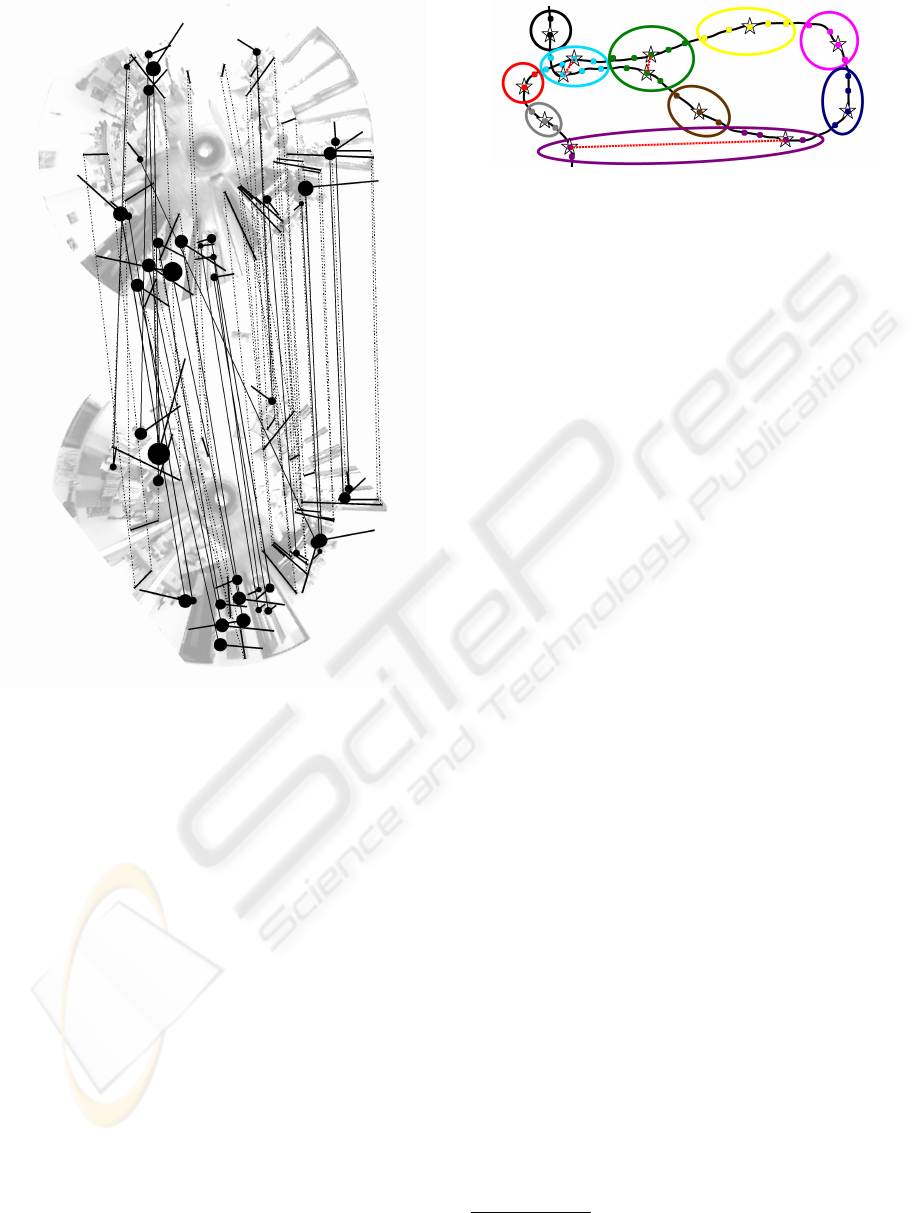
Figure 2: A pair of omnidirectional images, superimposed
with corresponding column segments (radial lines, matches
indicated with dotted line) and SIFT features (circles with
tail, matches with continues line). The images are rotated
for optimal visibility of the matches.
The dots in the sketch figure 3 denote places where
images are taken. Because they were taken at constant
time intervals and the robot did not drive at a constant
speed, they are not evenly spread. We perform an ag-
glomerative clustering with complete linkage based
on the visual distance (equation 4) on all the images,
yielding the ellipse shaped clusters in fig. 3. The black
line shows the exploration path as driven by the robot.
3.4 Hypothesis Formulation
As can be seen in the example (fig. 3), not all image
groups nicely cover one distinct place. This is due to
self-similarities, or distinct places in the environment
that are different but look alike and thus yield a small
visual distance between them.
For each of the clusters, we can define one or more
Figure 3: Example for the image clustering and hypothesis
formulation algorithms. Dots are image positions, black is
exploration path, clusters are visualised with ellipses, pro-
totypes of (sub)clusters with a star. Hypotheses are denoted
by a dotted red line.
subclusters. Images within one cluster who are linked
by exploration path connections are grouped together.
For each of these subclusters a prototype image is
chosen as the medoid
2
based on the visual distance,
denoted as a star in the figure.
As can be seen in the example, clusters containing
more than one subcluster can be one of two possibili-
ties:
- real loop closings, i.e. the robot is revisiting a place
and detected that it looks alike.
- erroneous self-similarities, i.e. distinct places that
look alike to the system.
For each pair of these subclusters within the same
cluster, we define a loop closing hypothesis H, which
states that if H = true, the two subclusters describe
the same physical place and must be merged together.
We will use Dempster-Shafer theory to collect evi-
dence about each of these hypotheses.
3.5 Dempster-Shafer Evidence
Collection
For each of the hypotheses defined in the previous
step, a decision must be made if it was correct or
wrong. Figure 4 illustrates four possibilities for one
hypothesis. We observe that a hypothesis has more
chance to be true if there are more hypotheses in the
neighbourhood, like in case a and b. If no neighbour-
ing hypotheses are present (c,d), no more evidence
can be found and no decision can be made based on
this data.
We conclude that for a certain hypothesis, a neigh-
bouring hypothesis adds evidence to it. It is clear that,
the further away this neighbour is from the hypothe-
sis, the less certain the given evidence is. We chose
to model this subjective uncertainty by means of the
ignorance notion in Dempster-Shafer theory. That is
2
The medoid of a cluster is analogous to the centroid,
but uses the median operator instead of the average.
ICINCO 2006 - ROBOTICS AND AUTOMATION
6
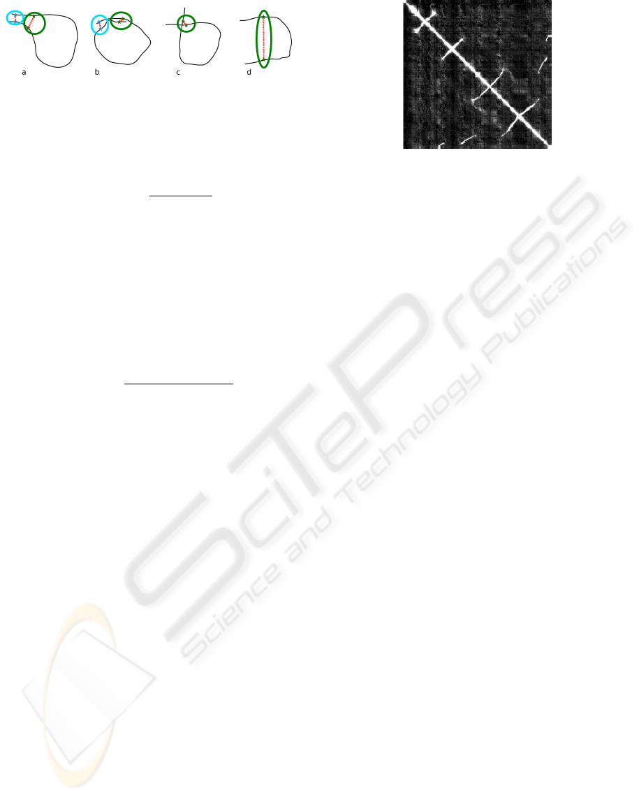
Figure 4: Four topological possibilities for one hypothesis.
why we define an ignorance function containing the
distance between two hypotheses H
a
and H
b
:
ξ(H
a
, H
b
) =
(
1 − sin
d
H
(H
a
,H
b
)π
2d
th
(d
H
≤ d
th
)
0 (d
H
> d
th
)
(5)
where d
th
is a distance threshold and d
H
(H
a
, H
b
) is
the sum of the distances between the two pairs of pro-
totypes of both hypotheses, measured in number of
exploration images.
To gather aleatory evidence, we look at the visual
similarity of both subcluster prototypes, normalised
by the standard deviation of the intra-subcluster visual
similarities:
s
V
(H
a
) =
s
V
(prot
a1
, prot
a2
)
σ
subclus
(s
V
)
, (6)
Where the visual similarity s
V
is derived from the vi-
sual distance, defined in equation 4.
Each neighbouring hypothesis H
b
yields the fol-
lowing set of Dempster-Shafer masses, to be com-
bined with the masses of the hypothesis H
a
itself:
m({∅}) = 0
m({H
a
}) = s
V
(H
b
)ξ(H
a
, H
b
)
m({¬H
a
}) = (1 − s
V
(H
b
))ξ(H
a
, H
b
)
m({H
a
, ¬H
a
}) = 1 − ξ(H
a
, H
b
)
(7)
Hypothesis masses are initialised with the visual sim-
ilarity of its subcluster prototypes and a initial igno-
rance value (0.25 in our experiments), which models
its influenceability by neighbours.
3.6 Hypothesis Decision
After combination of each hypothesis’s mass set with
the evidence given by neighbouring hypotheses (up to
a maximum distance d
th
), a decision must be made if
this hypothesis was correct and thus if the subclusters
must be united into one place or not.
Unfortunately, as stated above, only positive evi-
dence can be collected, because we can not gather
more information about totally isolated hypotheses
(like c and d in fig. 4). This not too bad, because of
different reasons. Firstly, the chance for correct, but
isolated hypothesis (case c) is low in typical cases.
Also, adding erroneous loop closings (c and d) will
yield an incorrect topological map, whereas leaving
Figure 5: Matrix showing the visual similarities between
the images of the experiment.
them out will keep the map useful for navigation, but
a bit less complete. Of course, new data about these
places can be acquired later, during navigation.
Important is to remind that the computed
Dempster-Shafer masses can not directly be in-
terpreted as probabilities. That is why we use
equation 3 to compute the support and plausibility of
each hypothesis after evidence collection. Because
these values define a confidence interval for the real
probability, a hypothesis can be accepted if the lower
bound (the support) is greater than a threshold.
After this decision, a final topological map can be
built. Subclusters connected with accepted hypothe-
ses are merged into one place, and a new medoid
is computed as prototype of it. For hypotheses that
are not accepted, two distinct places should be con-
structed.
4 EXPERIMENTS
With the camera system mounted on a electric wheel
chair (see fig. 1), we drove around in a complex nat-
ural environment, being our office floor. 463 images
were recorded during this path of 275 m length. Fig-
ure 6 shows a map of the environment. It can be seen
that the path visits several offices and corridors more
than once, generating the possibility for a lot of loop
closing hypotheses. Figure 7 gives a few typical im-
ages acquired.
Between each pair of images, fast wide baseline
features are matched and the proposed visual distance
measure is computed, yielding the similarity matrix
visualised in fig. 5. Based on this, the images are
clustered as shown with different symbols in fig. 6,
resulting in 38 clusters. For each subcluster, a pro-
totype is chosen denoted by a black star. Between
subclusters within one cluster, hypotheses are formu-
lated, denoted by thick black dotted lines.
As can be seen in the map, all but one hypothe-
sis (number 10) are correct. This is clearly a self-
similarity in the environment, the two offices do not
VISUAL TOPOLOGICAL MAP BUILDING IN SELF-SIMILAR ENVIRONMENTS
7
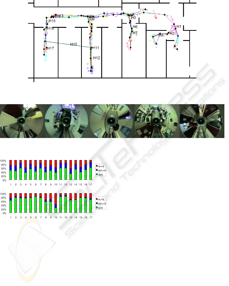
Figure 6: Right: Map of the experiment. Scattered datapoints are image positions, shown in various symbols denoting
clustering. Stars are (sub)clusters. The exploration path is visualised with thin black lines, hypotheses with thick dotted lines.
Figure 7: Images 256, 315, 345, 388 and 430 of the experiment.
Figure 8: Dempster-Shafer masses for each of the hypothe-
ses, before (above) and after (below) evidence collection.
differ enough in appearance. Figure 8 gives the
Dempster-Shafer masses of each hypothesis before
and after evidence collection. It is clear that after ev-
idence combination, we have more reason to reject
hypothesis 10.
The other subclusters can be merged, resulting in
the final topological map, shown in figure 9.
5 CONCLUSION
This paper described a method to find topological
loop closings in a sequence of images taken in a nat-
ural environment. The result is a vision-based topo-
logical map which can be used for localisation, path
planning and navigation.
Firstly, a robust visual distance was presented.
Making use of state-of-the-art wide baseline match-
ing techniques, this enables the recognition of places
despite changes in viewpoint, illumination, and the
presence of occlusions.
Secondly, a mathematical model is presented to
solve the problem of self-similarities, i.e. places in
the environment that look alike but are different. This
approach uses Dempster-Shafer probability theory to
combine evidence of neighbouring loop closing hy-
potheses.
The real-world experiments presented illustrate the
performance and robustness of the approach.
Future work planned includes the introduction
of even more performant visual features such as
SURF (Bay et al., 2006), and the on-line adaptation
of the map while using it for navigation.
ACKNOWLEDGEMENTS
This work is partially supported by the Inter-
University Attraction Poles, Office of the Prime Min-
ister (IUAP-AMS), the Institute for the Promotion of
ICINCO 2006 - ROBOTICS AND AUTOMATION
8
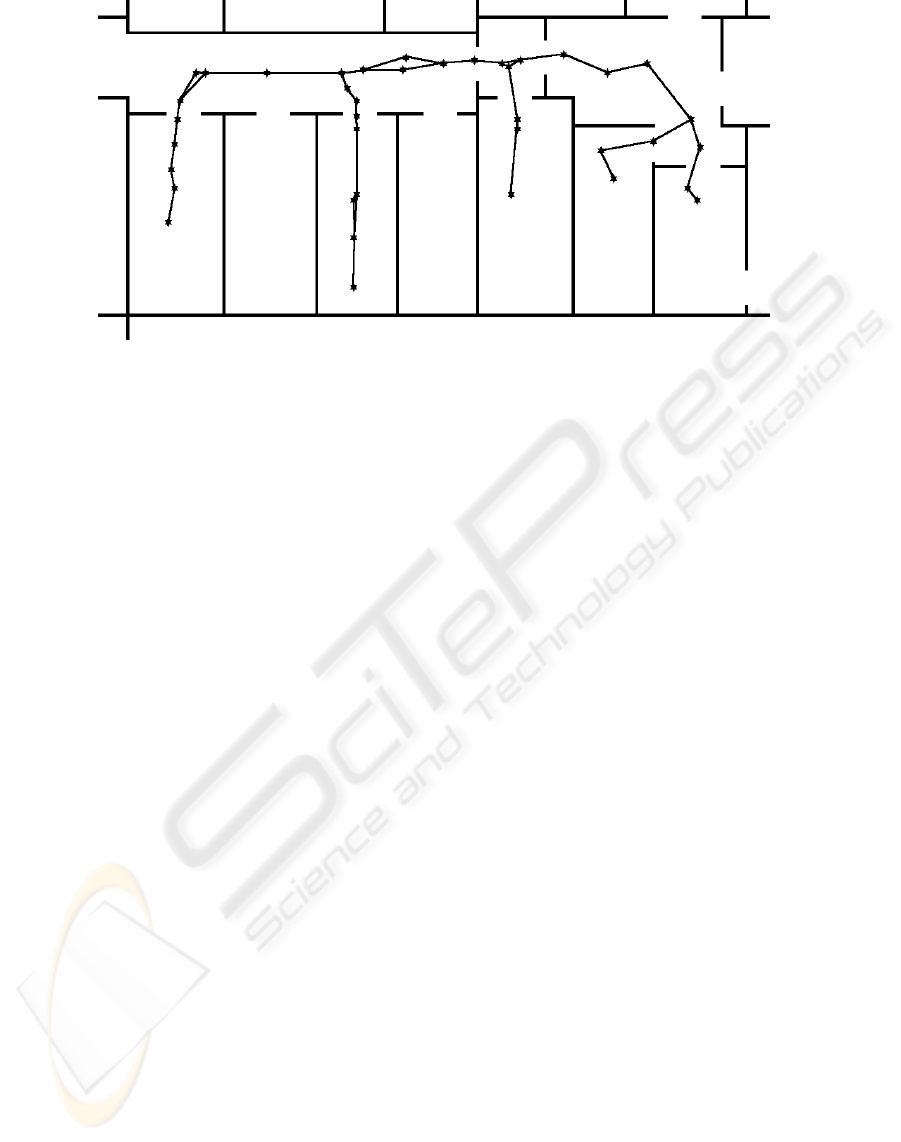
Figure 9: Final topological map. Stars denote prototypes.
Innovation through Science and Technology in Flan-
ders (IWT-Vlaanderen), and the Fund for Scientific
Research Flanders (FWO-Vlaanderen, Belgium).
REFERENCES
Bay, H., Tuytelaars, T., and Van Gool, L. (2006). Surf:
Speeded up robust features. In European Conference
on Computer Vision. In press.
Beevers, K. and Huang, W. (2005). Loop closing in topo-
logical maps. In ICRA.
Chen, C. and Wang, H. (2005). Appearance-based topolog-
ical bayesian inference for loop-closing detection in
cross-country environment. In IROS, pages 322–327.
Dempster, A. P. (1967). Upper and lower probabilities in-
duced by a multivalued mapping. In The Annals of
Statistics (28), pages 325–339.
Goedem
´
e, T., Nuttin, M., Tuytelaars, T., and Van Gool, L.
(2004a). Markerless computer vision based localiza-
tion using automatically generated topological maps.
In European Navigation Conference GNSS.
Goedem
´
e, T., Nuttin, M., Tuytelaars, T., and Van Gool,
L. (2004b). Vision based intelligent wheelchair con-
trol: the role of vision and inertial sensing in topolog-
ical navigation. In Journal of Robotic Systems, 21(2),
pages 85–94.
Goedem
´
e, T., Tuytelaars, T., and Van Gool, L. (2004c). Fast
wide baseline matching with constrained camera po-
sition. In Conference on Computer Vision and Pattern
Recognition, pages 24–29.
Goedem
´
e, T., Tuytelaars, T., Vanacker, G., Nuttin, M., and
Van Gool, L. (2005). Feature based omnidirectional
sparse visual path following. In International Confer-
ence on Intelligent Robots and Systems, IROS 2005,
pages 1003–1008.
Koenig, S. and Simmons, R. (1996). Unsupervised learning
of probabilistic models for robot navigation. In ICRA.
Lowe, D. (2004). Distinctive image features from scale-
invariant keypoints. In IJCV (60), pages 91–110.
Nagatani, K., Choset, H., and Thrun, S. (1998). Towards ex-
act localization without explicit localization with the
generalized voronoi graph. In ICRA, pages 342–348.
Ranganathan, A., Menegatti, E., and Dellaert, F. (2005).
Bayesian inference in the space of topological maps.
In IEEE Transactions on Robotics.
Shafer, G. (1976). A Mathematical Theory of Evidence.
Princeton University Press.
Shatkay, H. and Kaelbling, L. P. (1997). Learning topolog-
ical maps with weak local odometric information. In
IJCAI (2), pages 920–929.
Tapus, A. and Siegwart, R. (2005). Incremental robot map-
ping with fingerprints of places. In IROS.
Tolman, E. C. (1948). Cognitive maps in rats and men. In
Psychological Review (55), pages 189–208.
Tomatis, N., Nourbakhsh, I. R., and Siegwart, R. (2002).
Hybrid simultaneous localization and map building:
Closing the loop with multi-hypotheses tracking. In
ICRA, pages 2749–2754.
Wahlgren, C. and Duckett, T. (2005). Topological map-
ping for mobile robots using omnidirectional vision.
In SWAR.
Zivkovic, Z., Bakker, B., and Kr
¨
ose, B. (2005). Hierarchical
map building using visual landmarks and geometric
constraints. In IROS, pages 7–12.
VISUAL TOPOLOGICAL MAP BUILDING IN SELF-SIMILAR ENVIRONMENTS
9
