ELLIPTIC NET - A PATH PLANNING ALGORITHM FOR DYNAMIC

ENVIRONMENTS

Martin Saska

CTU in Prague, The Gerstner Laboratory for Intelligent Decision Making

Technicka 2, 16627 Prague 6, Czech Republic

Informatics VII: Robotics and Telematics, University Wuerzburg, Germany

Miroslav Kulich and Libor P

reu

cil

CTU in Prague, Center of Applied Cybernetics and The Gerstner Laboratory for Intelligent Decision Making

Technicka 2, 16627 Prague 6, Czech Republic

Keywords:

Path planning, Graph searching, Robotic soccer, Obstacle avoidance, Mobile robot, Ellipse.

Abstract:

Robot path planning and obstacle avoidance problems play an important role in mobile robotics. The standard

algorithms assume that a working environment is static or changing slowly. Moreover, computation time and

time needed for realization of the planned path is usually not crucial. The paper describes a novel algorithm

that is focused especially to deal with these two issues: the presented algorithm - Elliptic Net is fast and

robust and therefore usable in highly dynamic environments. The main idea of the algorithm is to cover an

interesting part of the working environment by a set of nodes and to construct a graph where the nodes are

connected by edges. Weights of the edges are then determined according to their lengths and distance to

obstacles. This allows to choose whether a generated path will be safe (far from obstacles), short, or weigh

these two criterions. The Elliptic Net approach was implemented, experimentally veriﬁed, and compared with

standard path planning algorithms.

1 INTRODUCTION

Trajectory planning is one of the most important parts

of every robotic system. A new approach for mobile

robots working in a highly dynamic environment is

presented in this paper.

Standard obstacle avoidance approaches ﬁnd a de-

sired path from an actual position S of the robot to

a desired goal position C, with respect to positions,

sizes, and shapes of known obstacles P in the envi-

ronment. The output of the algorithm can be either an

optimal trajectory connecting S with C (global algo-

rithms) or only direction from the actual position re-

specting locally optimal trajectory (local algorithms).

The basic requirement for the planned trajectory

is its optimality, which can be expressed as a length

of the trajectory or time needed to realize it. More-

over, the path should be easily feasible with respect

to both dynamic and kinematic constrains. In other

words, the path should be smooth path and does not

contain sharp turns. Unfortunately, ability to prevent

collisions is antagonistic to the requirement for path

optimality. Nevertheless, obstacle avoidance is nec-

essary, because collisions can cause damage of the

robot or obstacles and even endanger persons in ro-

bot’s workspace. To ﬁnd an acceptable compromise

between these requirements (the length and the dis-

tance to obstacles) is one of the most crucial problems

in mobile robot planning.

Standard algorithms described in the literature

cover whole workspace of the robot by a squared or

hexagonal grid which causes that dynamic features of

a robot are not respected. Another problem of stan-

dard approaches is big computational time. Such al-

gorithms cannot be used in dynamic environments,

where re-planning is invoked with high frequency.

In this paper, a novel method (called Elliptic Net)

is presented that avoids drawbacks mentioned in the

previous paragraph. The key idea of the approach is

to represent the working environment by a structure

based on a set of ellipses. Generated paths are then

smoother and more feasible. Moreover, the presented

approach takes into account only an interesting part

of the workspace that leads to reduction of computa-

tional time.

The rest of the paper is organized as follows. A

short review of the most popular obstacle avoidance

techniques is presented in the section 2, while a novel

method called Elliptic Net reﬂecting special require-

ments of the mobile robotics is described in section 3.

Finally, experimental results are described in section

4 and conclusions are presented in section 5.

372

Saska M., Kulich M. and P

reu

cil L. (2006).

ELLIPTIC NET - A PATH PLANNING ALGORITHM FOR DYNAMIC ENVIRONMENTS.

In Proceedings of the Third International Conference on Informatics in Control, Automation and Robotics, pages 372-377

DOI: 10.5220/0001208403720377

 SciTePress

2 LITERATURE SURVEY

Comprehensive review of path planning and obstacle

avoidance methods can be found in (Latombe, 1991).

Algorithms usually used in mobile robotics are di-

vided there into two types: local and global. Local

approaches ﬁnd only optimal direction from the ac-

tual position using information from a local area of

the robot. While locality of these approaches leads

to low computational time, generated trajectories are

not guaranteed to be globally optimal. Moreover, un-

availability of a full path can cause problems to low-

level regulators and strategy planning methods that

can need a full path for their better decision process.

Vector Field Histograms VFH (Borenstein and Ko-

ren, 1991), originally developed for obstacle avoid-

ance of robots equipped with sonars are a typical ex-

ample of local approaches. Similarly to a rotating

sonar exploring a space in 360 range, VFH obtains

histogram distances to the closest obstacle in each di-

rection. Directions whose distance is smaller than an

adaptive threshold are selected from this histogram.

Value of the threshold depends on a distance of the

robot to the goal position. The direction that has the

smallest angle to vector SC is chosen as optimal robot

heading. VFH cannot solve situations with high den-

sity of obstacles and with U-shape obstacles. Both

types of the workspace conﬁgurations caused move-

ments oscillation.

The most widely used collision avoidance method

is Potential Field (Khatib, 1986). It minimizes a

penalty function Z that consists of two parts. The re-

pulsive one describes inﬂuence of the obstacles in the

workspace, while the attractive part expresses inten-

tion to go to the desired point. In the other words, the

repulsive part discriminates paths that are close to ob-

stacles - it has a maximum in a centre of each obstacle

and decreases with a distance. The attractive part has

a global minimum in the goal of the robot and uni-

formly grows with a distance to the goal. The biggest

problem of this approach is that optimisation can ﬁn-

ish in a local minimum and therefore a globally opti-

mal path is not guaranteed to be found. The Potential

Field algorithm is used in this paper for comparison

with the following penalty function:

Z(x, y) =

(x − G

)

+ (y − G

)

(

x − A

−

x − B

y − A

y − B

) +

j=1

(exp(−c

((x − P

)

+ (y − P

)

))). (1)

G is the desired position of the robot, [P

, P

] are

coordinates of a center of j−th obstacle, A is a left

bottom corner of the playground (we suppose that the

workspace has a rectangular shape with boards along

it), B is a right top corner of the playground and c

are

constants weighting inﬂuences of the attractive and

repulsive parts.

Visibility Graph approach VG (Kunigahalli and

Russell, 1994) constructs a visibility graph (VG) of

vertices of polygons representing obstacles. It means

that two vertices are connected in VG if there are visi-

ble. A shortest path is then determined using standard

Dijkstra algorithm (Jorgen and Gutin, 1979). The

path found by this algorithm is typically close to the

obstacles, which often leads to collisions because ro-

bots cannot follow the planned path precisely. Grow-

ing of the obstacles by a certain value can solve this

problem, but it is not clear how to optimally determine

this value.

Occupancy Grid (Braunl and Tay, 2001) divides

a workspace into disjoint cells that cover the whole

space. The value of a cell is one if a part of any ob-

stacle is inside the cell or zero otherwise. Centres of

zero-valued cells are nodes of the graph, while edges

connect neighbouring nodes.

Voronoi Diagrams (VD) (Aurenhammer and Klein,

2000) divide a workspace into disjoint cells also.

Given a set P of points in the plane, one cell of VD is

a set of points that are closer to the speciﬁc point than

to any other point in P . For robotic purposes, the set

P contains centres of robots (excluding the one the

plan is generated for) plus points representing boards

around the playﬁeld. One possibility is to represent

each barrier by a set of points placed along each bar-

rier, but it increases computation time. The second

way is to compute generalized VD where the set P

can contain lines also. As it the previously mentioned

algorithms, a shortest path in the graph where neigh-

bouring cells of VD are connected can be found by

Dijkstra algorithm.

VD ﬁnd very safe paths, i.e. the paths are generated

as far as possible from obstacles. This is useful in

dense environments, while paths generated in sparse

spaces are needlessly long and cautious.

3 ELLIPTIC NET

In this section we introduce a novel obstacle avoid-

ance algorithm - Elliptic Net that is designed to have

a small computational complexity and to avoid disad-

vantages of above-described methods. The main idea

of the algorithm is to cover a whole working environ-

ment by a set of nodes and construct a graph, where

neighboring nodes are connected by an edge.

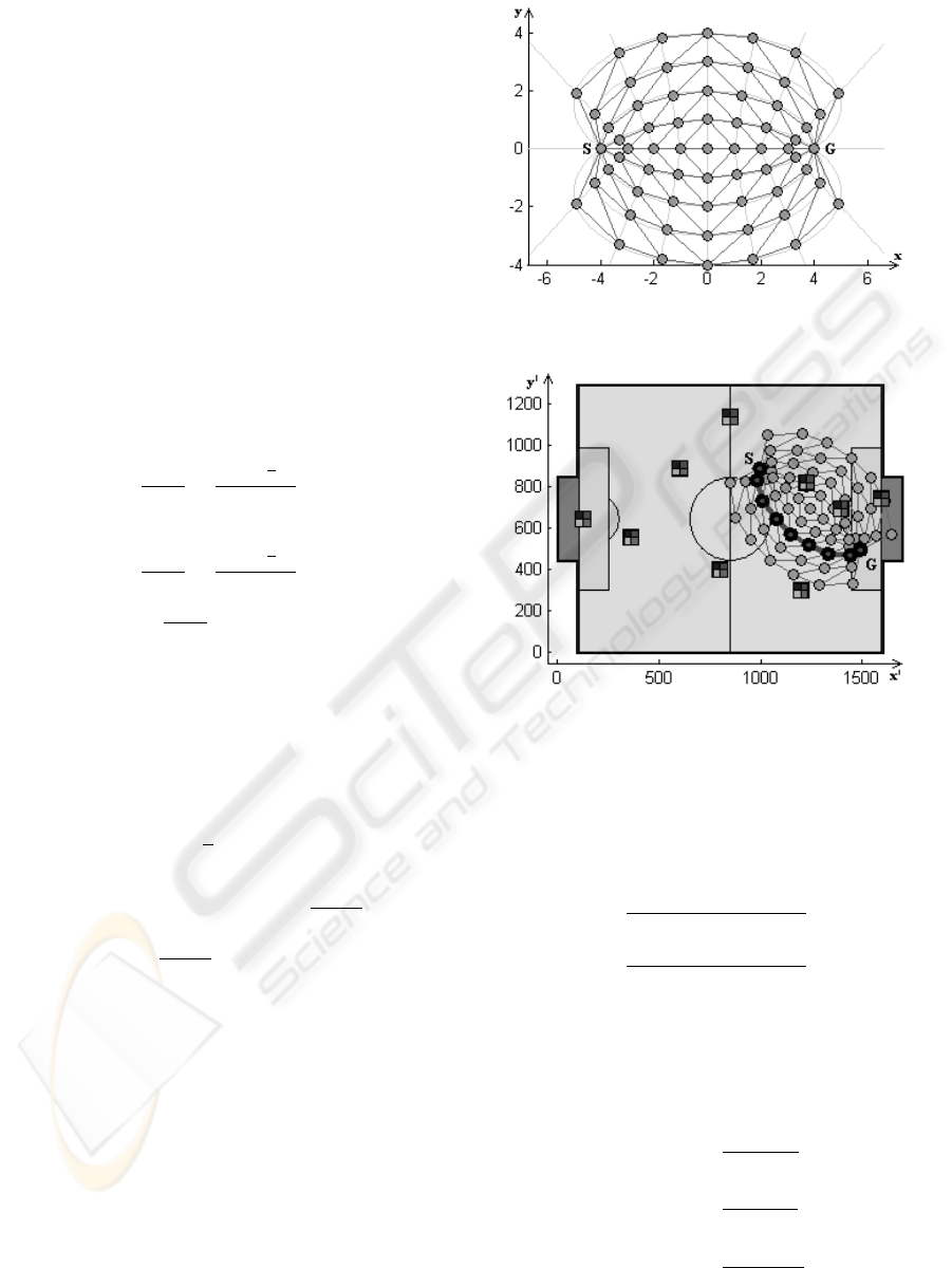
The algorithm consists of three main steps. In the

ﬁrst one, topology of the net is created in a general

position (see Figure 1). A number of points in the net

depends on a distance between the start and the goal

position. In order to increase a speed of the algorithm,

ELLIPTIC NET - A PATH PLANNING ALGORITHM FOR DYNAMIC ENVIRONMENTS

373

the net is not computed on the ﬂy. Instead of this,

several basic nets with a different number of points

are pre-computed. An appropriate net is then chosen

in a planning phase.

The net is then transformed (translated, rotated, and

resized) into a correct position according to the actual

and desired positions of the robot. Finally, weights

of edges in the graph are determined and the optimal

(according to the weights) path in the graph is found.

3.1 Net Description

Topology of the Elliptic Net is based on intersection

of a set of ellipses and a set of half-lines. i-th ellipse

is deﬁned by its centre E(i) and lengths of its axes a(i)

and b(i) that are given by the following equations:

(i) = 0, (2)

(i) =

i + 1

−

(w −

)

.(i + 1).p, (3)

a(i) = p.b(i), (4)

b(i) =

i + 1

(w −

)

.(i + 1).p, (5)

i ∈ 1..

t − 1

where p is ratio of the lengths of axes, w is a num-

ber of nodes lying on the line SG and t is a number of

nodes that lie on axis y. The half-lines are determined

by the equation y = kx+q. Parameters k(j) and q(j)

of j-th half-line are determined by equations

k(j) = tg(

u=1

(

)

), (6)

q(j) = −k(j).(−(j + 1) +

w − 1

), (7)

i ∈ 1..

w − 1

Intersection points of all ellipses and lines deﬁne

nodes of the Eliptic Net in one quarter of the plane.

Rest of the nodes is obtained as an axial symmetry

according to the axes x and y as shown in Figure 1.

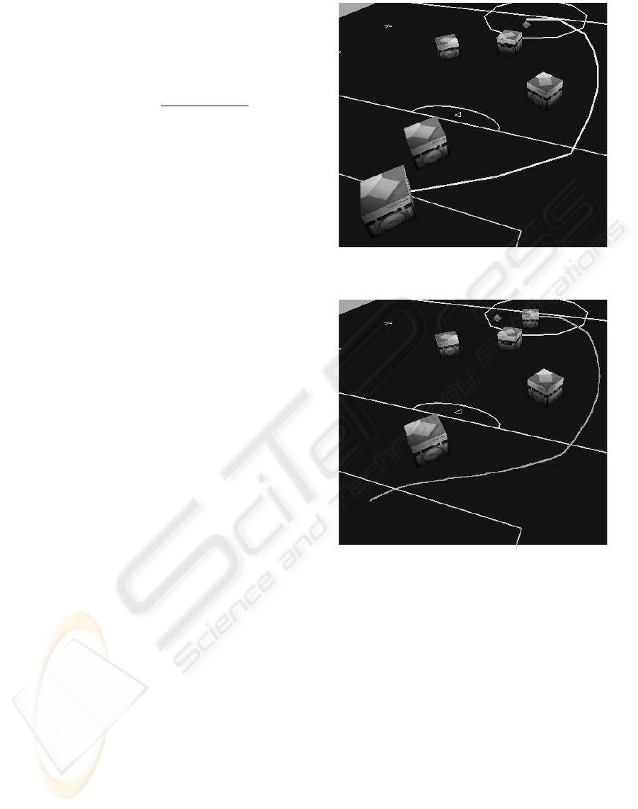
3.2 Transformed Net

In order to get optimal results, a distance between

neighbouring nodes should be comparable to the size

of obstacles. This requires generating a net with thou-

sands of edges to cover even a small area. Instead of

that only a grid of points covering the area along a

straight line connecting robot’s actual position with

the requested goal position is constructed.

Figure 1: Net in the basic form.

Figure 2: Net transformed to the correct position.

The net in a general position is transformed (ro-

tated, translated, and resized) to a correct position (see

Figure 2) according to the following equations:

′

x.cos(α) − y.sin(α)

+ S

, (8)

′

y.cos(α) − x.sin(α)

+ S

, (9)

where [x, y] are coordinates of a node in a pre-

deﬁned net, [x

′

, y

′

] coordinates in the resulting net,

[Sx, Sy] robot’s start position, and k and α scale and

rotation parameters, which are calculated as follows:

cos(α) =

− S

d(S, G)

, (10)

sin(α) =

− S

d(S, G)

, (11)

k =

(n − 1).g

d(S, G)

, (12)

where n is a number of nodes, which lie on the line

ICINCO 2006 - ROBOTICS AND AUTOMATION

374

SG and g stands for a distance between two neigh-

bouring nodes on SG.

Weights of edges are ﬁnally evaluated according to

their lengths and positions of obstacles:

w(e) = length(e).(1 +

j=1

d(C(e), C(o

))

), (13)

where length(e) is a length of edge e, d(.) stands

for Euclidean distance, C(e) is the center of e, C(o

)

is the center of obstacle o

, n is a number of obstacles

and c is a constant. This means that the closer an edge

lies to some obstacle the higher is its weight. The op-

timal trajectory is then the cheapest path in this graph

found by Dijkstra algorithm.

4 EXPERIMENTAL RESULTS

The functionality and the robustness of the Elliptic

Net algorithm has been experimentally veriﬁed. The

goal of the ﬁrst experiment was to set all constants in

an optimal way. The results of the experiment show

also inﬂuence of different settings of the parameters.

In the other part of testing, the Elliptic Net was com-

pared with two standard approaches often used in mo-

bile robotics. An experimental set of 1000 random

scenes was generated for both above-mentioned ex-

periments. Each scene contains 9 randomly generated

obstacles and random start and goal positions of the

robot. The set of scenes was a little bit reduced for

the second experiment ( see section 4.2).

The situations were solved by all algorithms and

the generated paths were evaluated and compared ac-

cording to several criteria (see Tables below). The

ﬁrst criterion l stands for a length of the path; the other

one d describes ability of the algorithm to ﬁnd a path

in safe distance from all obstacles. Precisely, it is the

shortest distance between any obstacle and the trajec-

tory. The values wc and hc mean a number of colli-

sions. The ”weak” collision wc occurs if d is smaller

than the robot radius. In this case the robot lightly

touches an obstacle and can push it. In the case d is

smaller than a half of the robot radius, we speak about

a ”hard” collision hc. The last, but one of the most

important criterion is t that describes computational

complexity. The complexity is described as a ratio of

time needed by the algorithm to time needed to solve

the same problem by Visibility Graph algorithm.

The third experiment consists in intensive testing

by simulations. The ﬁrst simulator (Krajn

ık et al.,

2006) that we used was robotic soccer simulator.

It can simulate real robot moving through the pre-

planned trajectory and collisions with obstacles (other

robots and barriers). Figure 3 shows one of the situa-

tions in the robotic soccer and the trajectory that was

Figure 3: Situation solved by Elliptic Net.

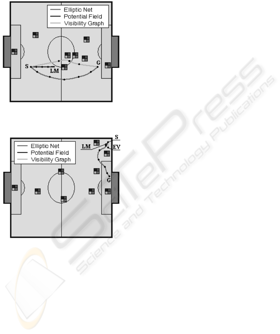
Figure 4: Simulated path to the desired position.

founded by Elliptic Net. The real path that robot go

through is visualized in the ﬁgure 4. Other simulation

contains of a trajectory generator that approximate the

founded trajectory by a spline curve that respects the

robot motions constraints. This approach is closely

described in (Saska et al., 2006) and some results for

all algorithms are shown in Figures 5,6.

4.1 Constants Setting

Inﬂuence of different settings of the constant c in

equation 13 on algorithm behavior that is evaluated

by indicators in Table 1 is described in this section.

Each row in the table shows values averaged for all

1000 situations from the experimental set.

Experiments show that the value of c can decide

whether the robot is controlled according safe (big c)

or fast (small c) strategy. In the ﬁrst case, distance

ELLIPTIC NET - A PATH PLANNING ALGORITHM FOR DYNAMIC ENVIRONMENTS

375

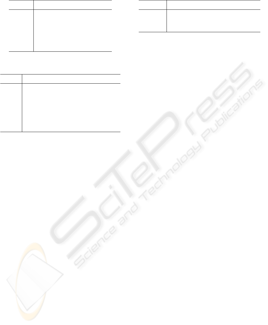
Table 1: Inﬂuence of constant c. Size of the net is 11x11.

c l[mm] d[mm] hc wc

500000 829.4 186.4 2 12

50000

819,2 183,9 1 10

25000

812,2 181,9 1 8

5000

742,6 156,6 9 102

2500

732,5 148,2 29 234

250

720,3 139,2 154 309

Table 2: Inﬂuence of size of the net. Constant c is 25000.

size l[mm] d[mm] hc w c t[%]

3x3 693,9 138,6 163 310 1,2

5x5

800,0 171,5 26 71 4,0

7x7

791,1 175,6 7 24 7,9

9x9

803,7 179,9 2 10 11,7

11x11

812,2 181,9 1 8 16,9

15x15

798,6 183,2 1 5 40,2

25x25

797,4 184,5 0 2 121,7

of a trajectory to obstacles increases and therefore the

number of collisions falls. It is caused by increas-

ing inﬂuence of obstacles, which ”pushes” a path to

the free space. A small value of c decreases distance

from the obstacles, but the trajectory is shorter and the

robot can reach the goal faster.

Relation among a size of the net, computational

time, and quality of the trajectory is evaluated in Ta-

ble 2. The rows depict different parameters according

to a number of nodes in the net. It can be stated that

nets with bigger than 7x7 produce remarkably smaller

number of paths with collisions. Interesting behav-

ior is shown in the second and third columns. These

two indicators are normally dependent in the sense

that a length of the path is increasing when a higher

safety is requested, which is not this case: with in-

creasing a net size, paths are shorter and more distant

from obstacles. This is caused by ﬁner resolution of

larger nets that allow controlling generated paths with

higher precision. On the other hand, time complexity

is of course higher for bigger nets, so sizes 9x9 and

11x11 looks as a good compromise between quality

of generated paths and time complexity.

4.2 Algorithm Comparison with

Other Methods

The algorithm Elliptic Net is compared in this section

with two standard methods described above - Poten-

tial Field and Visibility Graph. The experiment con-

sists of two parts. The same set as in the previous

section was used in the ﬁrst, but Potential Field ap-

Table 3: Different algorithms used for only 675 situations.

method l[mm] d[mm] wc nc t[%]

EN 741,5 205,2 0 7 28,4

711,1 203,2 0 1 1,8

667,0 175,1 0 134 100

proach was successful only in 675 situations, because

its optimization process can gets stuck in a local min-

imum. We therefore reduced the set to 675 situations

where the Potential Field gets results, otherwise the

results evaluated in Table 3 would be biased.

Visibility Graph has shortest average lengths (see

second column in the table), which corresponds with

expectations. Results obtained by the other ap-

proaches are nevertheless similar - they differ only by

4%. On the other hand, the trajectories found by the

Visibility Graph are too close to the obstacles, which

causes frequent crashes.

All situations used for the statistics in Table 3 were

solved without even weak collisions as shown in the

third column. That’s why we don’t use a number of

hard collisions as the other indicator, but a number of

trajectories nc that have a distance to the nearest ob-

stacle smaller than a robot radius multiplied by two.

20% of paths generated by the Visibility Graph algo-

rithm were dangerously near to obstacles, while other

two methods give signiﬁcantly better results.

The last indicator in the sixth columns is computa-

tional time. The Potential Field is fastest according to

this criterion, but the value in the table describes time

needed to ﬁnd only optimal robot’s heading instead

of the whole trajectory. If we use full version of the

algorithm generating whole trajectory, computational

time increases dramatically and it is then longer than

time needed by the Visibility Graph. The Elliptic Net

with 13x13 nodes is 3.5 times faster than the Visibility

Graph.

In the second part of the comparative experiments,

all algorithms were veriﬁed and their behaviour com-

pared on two types of simulations. Figure 5 shows

the ability of the Elliptic Net to avoid a cluster of the

obstacles. On the contrary, A trajectory found by the

Visibility Graph goes through this cluster. The path is

also too close to the obstacles, which can lead to col-

lision in case of odometry or control error or sudden

moving of the obstacle. Other important advantage

of the Elliptic Net is illustrated in Figure 6. This ap-

proach ﬁnds an optimal solution if a free path without

collision does not exist. The Visibility Graph is dis-

connected in such case and an optimal trajectory is

not found. The Potential Field gets stuck in the local

minimum in the same way as in the previous situation.

Paths generated by the algorithms were smoothed

by the spline generator and ﬁnal trajectories executed

ICINCO 2006 - ROBOTICS AND AUTOMATION

376

by the robot in the simulator were drown in both situ-

ations.

Figure 5: Situation solved by different algorithms.

Figure 6: Situation solved by different algorithms.

5 CONCLUSION

The Elliptic Net described in this paper is a novel

path planning algorithm that can be used in simple,

but dynamic environments. The optimal path is found

on a graph, whose nodes are determined as intersec-

tion of a specially created set of ellipses with a set of

half-lines. Most of the ﬁnal trajectories are smooth,

i.e. without sharp curves and a robot can follow the

planned path quickly.

This approach needs less computational time than

the other global algorithms and therefore it is accept-

able in highly dynamic environments where frequent

re-planning is needed. Local algorithms are of course

faster, but they have problems with clusters of the ob-

stacles and with local extremas. Quickly moving ob-

stacles are the reason, why the algorithm tries to avoid

them with sufﬁcient distance. Other important advan-

tage is its robustness. Algorithm has the ability to ﬁnd

some trajectory if a free path without collision doesn’t

exist. Like in a real life, it holds that bad decision is

better than no decision.

In the future, we would like to incorporate dynamic

obstacles directly into the algorithm. The idea is to

predict positions of obstacles (other robots) accord-

ing to their current states and situation on the ﬁeld

and evaluate edges in the planning graph according to

these predictions.

ACKNOWLEDGEMENTS

The work has been supported within the Czech-

Slovenian intergovernmental S&T Cooperation Pro-

gramme under project no. 10200506 ”Cooperative

mobile robots for industry and service”. The support

of the Ministry of Education of the Czech Republic,

under the Project No. 1M0567 to Miroslav Kulich is

also gratefully acknowledged.

REFERENCES

Aurenhammer, F. and Klein, R. (2000). Voronoi diagrams..

pages 201–290.

Borenstein, J. and Koren, Y. (1991). The vector ﬁeld his-

togram: Fast obstacle avoidance for mobile robots.

IEEE Journal of Robotics and Automation.

Braunl, T. and Tay, N. (2001). Combining conﬁgura-

tion space and occupancy grid for robot navigation.

28(3):233–41.

Jorgen, B. and Gutin, G. (1979). Digraphs: Theory, Algo-

rithms and Applications. Elsevier North Holland.

Khatib, O. (1986). Real-time obstacle avoidance for manip-

ulators and mobile robots. The International Journal

of Robotics Research, 5:90–98.

Krajn

ık, T., Faigl, J., and P

reu

cil, L. (2006). Decision sup-

port by simulation in a robotic soccer domain. In

MATHMOD 2006, ARGESIM-Reports.

Kunigahalli, R. and Russell, J. (1994). Visibility graph ap-

proach to detailed path planning in cnc concrete place-

ment.

Latombe, J. (1991). Robot Motion Planning. MA: Kluwer,

Norwell.

Saska, M., Kulich, M., Klancar, G., and Faigl, J. (2006).

Transformed net - collision avoidance algorithm for

robotic soccer. In MATHMOD 2006.

ELLIPTIC NET - A PATH PLANNING ALGORITHM FOR DYNAMIC ENVIRONMENTS

377