OPTICAL FLOW NAVIGATION OVER

ACROMOVI ARCHITECTURE

Patricio Nebot and Enric Cervera

Robotic Intelligence Lab

Campus de Riu Sec, E-12071 Castell

on de la Plana, Spain

Keywords:

Mobile robots, Multiagent systems, Optical ﬂow, Motion parameters, Obstacle avoidance.

Abstract:

Optical ﬂow computation involves the extraction of a dense velocity ﬁeld from an image sequence. The pur-

pose of this work is to use the technique of optical ﬂow so that a robot equipped with a color camera can

navigate in a secure way through an indoor environment without collide with any obstacle. In order to im-

plement such application, the Acromovi architecture has been used. Acromovi architecture is a distributed

architecture that works as middleware layer between the robot architecture and the applications, which al-

lows sharing the resources of each robot among all the team. This middleware is based on an agent-oriented

approach.

1 INTRODUCTION

During years, the problem of processing image se-

quences for calculating the optical ﬂow has been stud-

ied. The optical ﬂow can be used in many appli-

cations, but recently it has been applied in mobile

robot navigation (R. Carelli, 2002) (M. Sarcinelli-

Filho, 2002).

The optical ﬂow is the distribution of the apparent

velocities of movement of the brightness pattern in an

image, and arises from the relative movement of some

objects and a viewer (Horn and Schunck, 1981). As

the robot is moving around, although the environment

is static, there is a relative movement between the ob-

jects and the camera onboard the robot.

The visual information coming from the camera

of the robot is processed through the optical ﬂow

technique, which provides the information the robot

needs to safely navigate in an unknown working-

environment.

From the optical ﬂow generated in this way the

robot can get an inference on how far an object

present in a scene is. This information is embedded in

the time to crash (or time to collision) calculated from

the optical ﬂow ﬁeld (M. Sarcinelli-Filho, 2004).

The purpose of this work is to use the optical ﬂow

technique to allow a mobile robot equipped with a

color camera navigates in a secure way through an in-

door environment without collide with any obstacle.

2 DESCRIPTION OF THE

ACROMOVI ARCHITECTURE

As has been shown in previous works and papers,

Acromovi architecture is a distributed architecture for

programming and controlling a team of multiple het-

erogeneous mobile robots that are capable to cooper-

ate between them and with people to achieve service

tasks in daily environments.

This architecture allows the reutilization of code,

due to the use native components. It allows the shar-

ing of the robots’ resources among the team and an

easy access to the robots’ elements by the applica-

tions. And other two important characteristics of the

Acromovi architecture are the scalability and the fa-

cility of use.

Moreover, Acromovi architecture is a framework

for application development by means of embedding

agents and interfacing agent code with native low-

level code. Cooperation among the robots is also

made easier in order to achieve complex tasks in a

coordinated way. Also, Acromovi architecture is a

distributed architecture that works as a middleware of

another global architecture for programming robots.

This middleware is based on an agent-oriented ap-

proach. The embedded agents that constitute the

Acromovi architecture work as interfaces between the

applications and the physical elements of the robots.

Some agents also make easier the handle of these ele-

500

Nebot P. and Cervera E. (2006).

OPTICAL FLOW NAVIGATION OVER ACROMOVI ARCHITECTURE.

In Proceedings of the Third International Conference on Informatics in Control, Automation and Robotics, pages 500-503

DOI: 10.5220/0001207805000503

 SciTePress

ments and provide higher-level services.

This middleware level has been divided into two

layers. In the lower layer, there are a set of compo-

nents that access to the physical parts of the robots

and other special components that offer services to the

upper layer. The upper layer comprises a variety of

embedded agents addressed to supervise and control

the access to the agents of the lower layer.

3 BACKGROUND THEORY

3.1 Optical Flow

Optical ﬂow computation consists in extracting a

dense velocity ﬁeld from an image sequence assum-

ing that intensity or color is conserved during the dis-

placement. This result may be used by other appli-

cations like 3D reconstruction, time interpolation of

image sequences using motion information, segmen-

tation and tracking (Qu

enot, 1996).

The optical-ﬂow ﬁeld used in this work is obtained

by using formulas and constraints used by Horn and

Schunck (Horn and Schunck, 1981). The equation

that relates the change in image brightness at a point

to the motion of the brightness pattern is:

u + E

v + E

= 0 (1)

where, E(x,y,t) represents the value of brightness

at time t of a point with coordinates (x,y) in the image

plane. Ex, Ey, Et represent the partial derivatives of

E with relation to x, y, t respectively. u, v denote the

components of optical ﬂow along x and y respectively.

3.2 Time to Contact

A primary use of optical ﬂow is collision detec-

tion, in particular time-to-contact computation. Us-

ing only optical measurements, and without knowing

ones own velocity or distance from a surface, it is pos-

sible to determine when contact with a visible surface

will be made (Camus, 1995).

Figure 1: Optical geometry for time-to-contact.

A point of interest P at coordinates (X, Y, Z) is pro-

jected through the focus of projection centered at the

origin of the coordinate system (0,0,0). P is ﬁxed in

physical space and does not move. The origin /focus

of projection however moves forward with velocity

dZ/dt. If the camera is facing the same direction as

the direction of motion, then this direction is what is

commonly known as the focus of expansion (FOE),

since it is the point from which the optical ﬂow di-

verges. The image plane is ﬁxed at a distance z in

front of origin.: for convenience, we set z=1 (The ac-

tual value of z depends on focal length of camera). P

projects onto point p in this plane. As the image plane

moves closer to P, the position of p in the image plane

changes as well. Using equilateral triangle:

y/z = y/1 = Y/Z (2)

Differentiating with respect to time, we get:

y/ ˙y = −(Z/

Z) =τ (3)

The quantity τ is known as the time-to-contact.

Note that the left-hand side contains purely optical

quantities, and that knowledge of τ does not provide

any information about distance and velocity, but only

of their ratio.

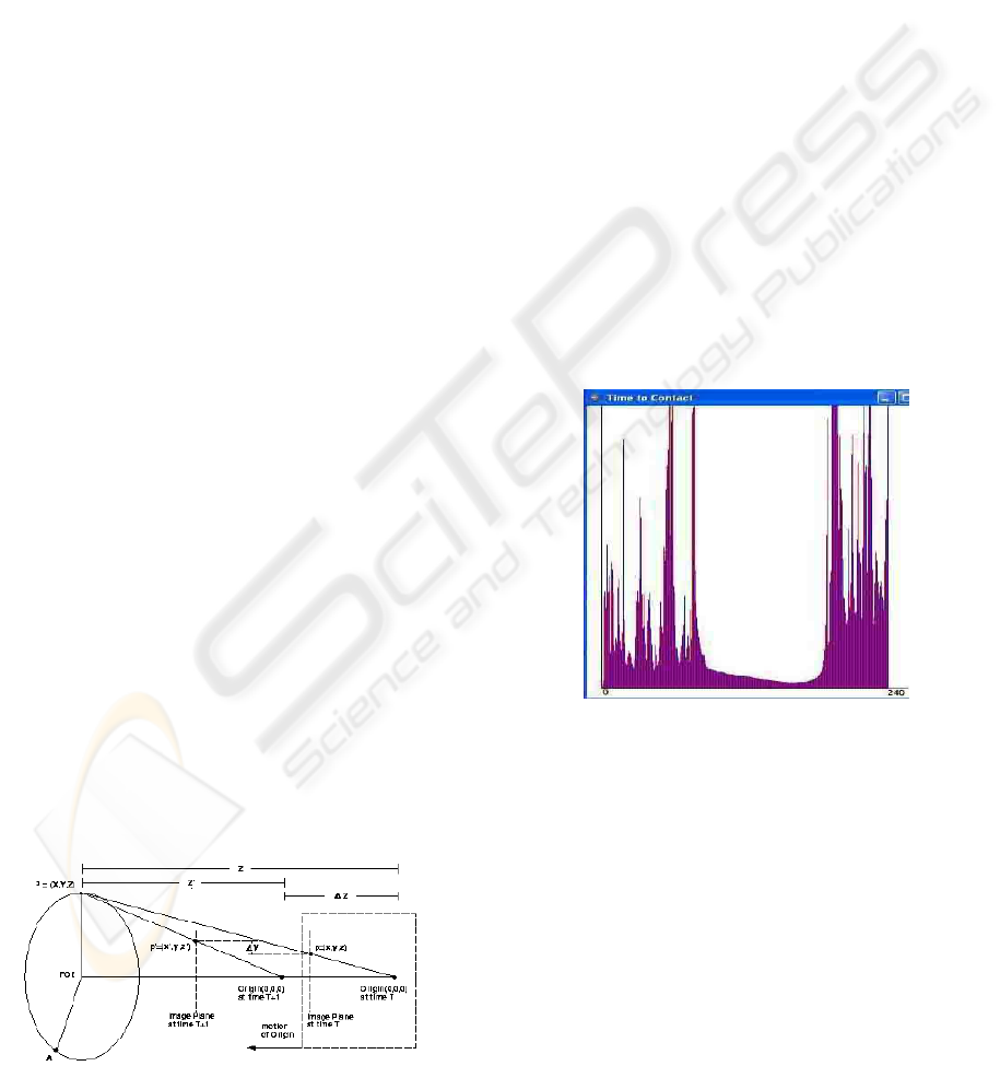
Figure 2: Example of time-to-contact graphic.

Based on the optical-ﬂow ﬁeld obtained as de-

scribed above, the sensing subsystem delivers to the

control subsystem information on the time to collision

corresponding to distinct stripes in the visual ﬁeld of

the robot, that can be seen in Fig. 2. In addition to the

vector of times to collision itself, the average value

and the standard deviation corresponding to its ele-

ments are also calculated.

3.3 Control System

Regarding the time-to-contact results shown in Fig. 2

and the additional information associated to them,

three different situations are considered here when

OPTICAL FLOW NAVIGATION OVER ACROMOVI ARCHITECTURE

501

implementing a system to control the heading angle

of the robot. They are labeled Imminent Collision,

Side Obstacle and Normal situations.

Imminent Collision is characterized either when

the average value and the standard deviation associ-

ated to the values of time to collision are both very

small (meaning that a wide object is very close to

the robot), or when an object for which the num-

ber of time-to-contact values inferior to the threshold

adopted is greater than another threshold is detected

in the middle of an image frame.

However, if an object for which the number of

time-to-contact values that are less than the threshold

adopted is greater than another threshold is detected

in the right side or in the left side of the visual ﬁeld of

the robot, the situation named Side Obstacle is char-

acterized.

Finally, the Normal situation is characterized when

no objects with high average optical ﬂow magnitude

are detected in the image frame. This means that all

objects in the visual ﬁeld of the robot are not close

enough to deserve an abrupt manoeuvre.

4 SYSTEM DEVELOPMENT

Three new agents have been designed for the develop-

ment of this application, the Vision Agent, the Opti-

calFlow Agent, and the Control Agent. Each of these

agents implements each of the modules described in

previous sections. A diagram of the relation among

these agents can be seen in Fig. 3.

Figure 3: Interaction among the agents.

The ﬁrst agent involved in the process is the JMF

Agent, which is in charge of capturing the input image

frames. The video from the camera on board the robot

is captured using the Java Media Framework (JMF).

Then, this image is sent to the next agent in the

process, the OpticalFlow Agent. This agent performs

two different works. Firstly, it calculates the optical

ﬂow derived from the new image, using the formulas

described above. Then, it calculates, from the optical

ﬂow, the time-to-contact vector, using also the formu-

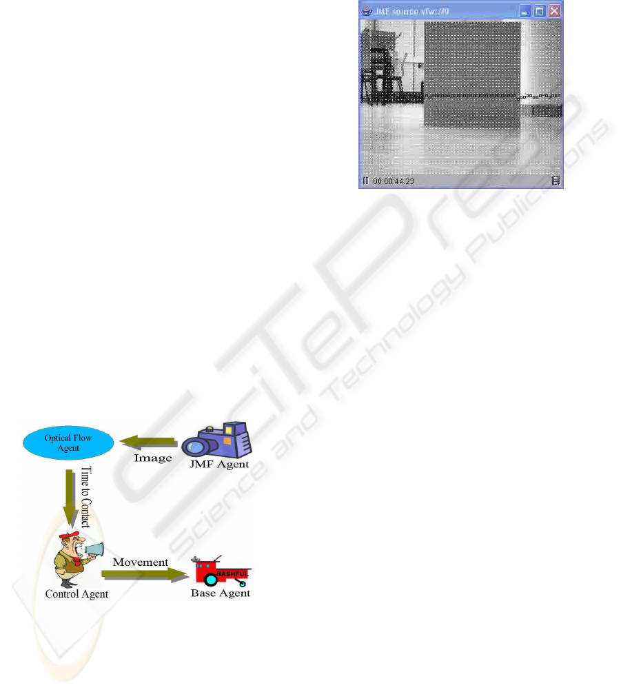
las described above in the article. In Fig. 4, there is

an example of the optical-ﬂow ﬁeld and in the Fig. 2,

the time-to-contact graphic.

Figure 4: Optical ﬂow ﬁeld.

Next, the OpticalFlow Agent sends the information

corresponding to the time to contact to the Control

Agent. This agent, depending on the graphic, can dis-

tinguish three distinct situations, as it has been said

above. These situations are Imminent Collision, Side

Obstacle, and Normal situations. Depending on the

situation that the Control Agent recognizes, it sends

different actions to the Base Agent, in order to the

robot can avoid an obstacle or can follow its way.

The Imminent Collision situation is done when an

object is in the middle of the image frame. That is, the

elements 80 to 160 of the vector of times to collision

have the values less than the others. In such cases, the

actions the Control Agent sends to the Base Agent are

to go back about 10 cm, to rotate 180 degrees and to

move ahead again.

The Side Obstacle situation is done when an object

is in the right or in the left side of the image frame.

The obstacle is in the right side when the elements

160 to 240 have the smaller values, and it is in the

left side when the elements 0 to 80 have the smaller

values. In such cases, the manoeuvre adopted sent to

the Base Agent is to rotate 15 degrees in the opposite

direction and to resume moving ahead.

Finally, the Normal situation is executed when no

object is in the image frame. In this case, all the ele-

ments of the vector of times to collision have similar

values. So, the command sent to the Base Agent is to

continue moving straight ahead.

It is important to remark that the time spent in cal-

culating the three parameters needed to the execution

of the application (the average value and the standard

deviation associated to the 240 values of time to colli-

sion used to build the graphic of Fig. 4 and the average

value of the magnitude of the optical ﬂow vectors as-

ICINCO 2006 - ROBOTICS AND AUTOMATION

502

sociated to each object detected in the scene) is very

small, not decreasing the capability of the robot to re-

act in real-time.

5 EXPERIMENTAL RESULTS

In order to check the performance of the robot when

wandering in its working-environment using the sens-

ing and control subsystems discussed here the robot

is programmed to wander around the lab, avoiding all

the obstacles it detects.

The robot used for it is a Pioneer2 mobile robot

with an onboard computer based on the Intel Celeron

650 MHz processor, having 508 Mbytes of RAM

memory. A Logitech web camera is also available

onboard the robot. The image capturing program in

java grabs the images that are at most 320x240 pixels

bitmaps at 5 fps in Linux platform.

An analysis of all the actions the robot has taken

shows that it was effectively able to avoid the obsta-

cles that appeared in its way, as expected, using the

time-to-contact based sensorial information.

As mentioned above, the robot acquires image

frames continuously at the interval of 200 ms, the cal-

culation of the optical ﬂow vectors plus the calcula-

tion of the new heading angle is compatible with the

rate of acquisition of images, thus showing that the

use of optical ﬂow for this kind of sensing is suitable.

In order to synchronize the calculation with the image

acquisition time, an image of 240x180 pixels is used.

6 CONCLUSIONS AND FUTURE

WORK

New agents have been implemented based on the

Acromovi architecture to make feasible that the robot

can navigate in an environment using the optical ﬂow

technique. These agents have been implemented

taking into account the limited computational setup

available onboard the robot.

The experimental results have shown that the robot

is effectively able to avoid any obstacle, in real-time,

based only on the information from the optical-ﬂow

and the time-to-contact agents.

Regarding the future work to do with the described

system, ﬁrst, sonars will be also used to distinguish

those situations in which an object is too close to the

robot and permits the robot to realize the evasive ma-

noeuvre. Another important improvement is to try to

change from the wander behaviour to a most reliable

navigation, following a speciﬁc path or trying to get

to a speciﬁc point in the working-environment.

It is important to try of reducing the time consump-

tion by the calculation of the optical ﬂow. For that,

it can be used new methods faster than the used in

this work. One possible option that implies a little

variation over the original method is the described in

(D.F. Tello, 2005). So, with a few changes it is pos-

sible to get a system faster and capable to react in a

more reliable way to changes in the environment.

Finally, this work can be extended to a team of

robots that can cooperate so that a certain robot with-

out the needed resources could navigate using the op-

tical ﬂow technique can do it. This can be possible

thanks to one of the advantages of the Acromovi ar-

chitecture, the possibility to share resources among

the robots of the team.

ACKNOWLEDGEMENTS

Support for this research is provided in part by ”Min-

isterio de Educaci

on y Ciencia”, grant DPI2005-

08203-C02-01, and by ”Generalitat Valenciana”,

grant GV05/137.

REFERENCES

Camus, T. (1995). Calculating time-to-contact using real-

time quantized optical ﬂow. In National Institute of

Standards and Technology NISTIR 5609.

D.F. Tello, e. a. (2005). Optical ﬂow calculation us-

ing data fusion with decentralized information ﬁlter.

In Proceedings of IEEE International Conference on

Robotics and Automation (ICRA 2005).

Horn, K. and Schunck, B. (1981). Determining optical ﬂow.

Artiﬁcial Intelligence, 17:185–203.

M. Sarcinelli-Filho, e. a. (2002). Using optical ﬂow to con-

trol mobile robot navigation. In Proceedings of the

15th IFAC World Congress on Automatic Control.

M. Sarcinelli-Filho, e. a. (2004). Optical ﬂow-based reac-

tive navigation of a mobile robot. In Proceedings of

the 5th IFAC/EURON Symposium on Intelligent Au-

tonomous Vehicles.

enot, G. (1996). Computation of optical ﬂow using dy-

namic programming. In Proceedings of International

Workshop on Machine Vision Applications.

R. Carelli, e. a. (2002). Stable agv corridor navigation with

fused vision-based control signals. In Proceedings of

the 28th Annual Conference of IEEE Industry Elec-

tronics Society.

OPTICAL FLOW NAVIGATION OVER ACROMOVI ARCHITECTURE

503