TOWARD 3D FREE FORM OBJECT TRACKING USING SKELETON

Djamel Merad

LIRIS laboratory

5 avenue Pierre Mendes-France, 69676 Bron

Jean-Yves Didier

LSC Laboratory

40 , Rue du Pelvoux, 91020 Evry Cedex

Keywords:

Tracking, 3D free form object, Skeletonization, Graph matching.

Abstract:

In this paper we describe an original method for the 3D free form object tracking in monocular vision. The

main contribution of this article is the use of the skeleton of an object in order to recognize, locate and track

this object in real time. Indeed, the use of this kind of representation made it possible to avoid difﬁculties

related to the absence of prominent elements in free form objects (which makes the matching process easier).

The skeleton is a lower dimension representation of the object, it is homotopic and it has a graph structure.

This allowed us to use powerful tools of the graph theory in order to perform matching between scene objects

and models (recognition step). Thereafter, we used skeleton extremities as interest points for the tracking.

1 INTRODUCTION

Object tracking is an important ﬁeld of artiﬁcial vi-

sion. It is a difﬁcult problem involved in tasks as mo-

tion evaluation or automatic visual control. The possi-

ble application are from medical imagery to security,

including the road trafﬁc analysis, etc.

The most part of algorithms allowing 3D pose esti-

mation from a 2D images sequence are based on the

same principle. The ﬁrst step consists in recognizing

the type of target in order to choose the best model

from a database (initialization). The second step, per-

formed during the treatment, consists in target track-

ing.

An initial pose of the objet is known either by an

initialization process before tracking, or by a predic-

tion process using the results obtained from the pre-

vious image. This initial pose allows to project the

target’s model onto the image’s plane. Starting from

this projection, it is possible to know if the pose is

good or not. A comparison measure between the 2D

image and the projected model allows a pose adjust-

ment (ﬁtting).

The general principle of tracking is common to all

the methods. Nevertheless they signiﬁcantly vary ac-

cording to their matching method or prediction tech-

niques. Among the different existing tracking meth-

ods, we will cite the one of Lowe (Lowe, 1992)

(Lowe, 1987) , of Gennery (Gennery, 1982) (Gennery,

1992) and of Harris (Harris and Stennet, 1990) which

we can qualify as generic methods. These three track-

ing methods give very good performances and use al-

gorithms of different complexities.

Some other methods were developed since. Some

model based approaches use the automatic visual con-

trol to track the salient edges of a model (Drum-

mond and Cipolla, 2002) while some other methods

use primitives as points, lines, or ellipses (Marchand

et al., 1999) (Comport et al., 2003). However, the pre-

sented methods were been developed for polyhedral

models having straight edges, which facilitate their

detection. That is the reason why these methods can

not be applied on free form object tracking.

To track free form objects, some methods use a pri-

ori and a posteriori information. These methods either

will index several images (shots) of the target object

depending on some points of interest and stock them

in a database, or will build a model starting from this

camera shot. The objets are tracked using ”patches”

together with the indexed images for a homographi-

cal matching (Vacchetti et al., 2004). Another way

to manage free form object tracking is to use a poor

sparse metric environment model in order to perform

real time model tracking using the camera (Skrypnyk

and Lowe, 2004). Unfortunately, these systems need

a learning step on several shots of the real object, they

can not use the 3D model only.

The most of the effective tracking methods were

Merad D. and Didier J. (2006).

TOWARD 3D FREE FORM OBJECT TRACKING USING SKELETON.

In Proceedings of the Third International Conference on Informatics in Control, Automation and Robotics, pages 74-81

DOI: 10.5220/0001207400740081

 SciTePress

developed for polyhedral objects. It would be enough

to extract a polyhedral primitive of our free form ob-

ject and to adapt the existing tracking algorithms. We

succeeded by using skeletons for the free form ob-

ject representation. Indeed, a skeleton is an object

representation in an inferior dimension. It has the ad-

vantage to preserve the most of the topological and

geometrical information of the silhouette. The skele-

tonization or the object representation by a set of seg-

ments, allows us to bypass the problem related to free

form objects.

In image processing and computer vision in gen-

eral, there are many applications for 2D and 3D ob-

jects skeletons (encoding, compression etc.). Further

to our interesting results obtained with this formalism

in free form object recognition and localization , we

explored its application to tracking this kind of ob-

jects.

More precisely, we adapted the Lowe method

(Lowe, 1992) to track a 2D skeleton using a 3D skele-

ton, therefore to track a 3D object in a 2D shot. The

points of interest we used are the two skeleton extrem-

ities. The initialization step corresponds to the target

pose computing, without any a priori knowledge of

the scene. The initialization system is described in

section (2) . Once the initial position of our object

known, it is possible to start tracking.

The 3D skeleton is projected on the image plane,

starting from its initial position, by using previously

calculated rotation and translation matrices. The algo-

rithm uses the fact that there is a small displacement

between two consecutive images in a video. There-

fore the positions of 2D skeleton points in two images

will be very close. A comparison measure between

the 2D skeleton of the image and the projected 3D

skeleton of the model is used for a pose adjustment.

This step is presented in section 3 and the obtained

results are presented in section 4.

2 INITIALISATION

In this section we present the identiﬁcation and the lo-

calization of 3D free form objects, starting from a 2D

image of scene, where partial occlusions may appear.

We analyzed the architecture of 3D free form more

popular recognition systems and we noticed the difﬁ-

cult problems to which they are confronted with.

Some of these difﬁculties are: to build the model

for complex objects, primitive extraction allowing a

correct matching and the lack of salient elements al-

lowing a robust pose estimation. We also can cite

complexity and occlusion problems which have not

a satisfactory solution.

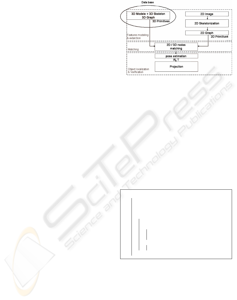
The approach we developed (ﬁgure 1), is based on

using a 3D skeleton of an a priori known model and

Figure 1: 3D free form object recognition by using skele-

tons.

the on-line extraction of the 2D skeleton of an image

of the object in front of the camera. The utilization

of this formalism allowed us to solve the problems

presented before: pose estimation and robustness to

occlusions and auto-occlusions. Our method is essen-

tially composed of three phases.

• Primitives modelization and extraction: search for

an appropriate representation and primitive detec-

tion in the image/model.

• Matching: search of the appropriate model for cor-

responding primitives

• Localization and veriﬁcation: matching validation

and pose estimation.

1. RecoginitionSystem (image I, {3DGraph G

}):

S ←− Skeletonization (I);

←− SkeletonToGraphTransform(S);

hypothesis ←− Indexation(G

, {G

});

for each h from {hypothesis} do

′

←− HypothesisChecking(G

, h);

if h

′

6= null then

OverlayImageWithModel;

exit;

10.

else

11.

h ←− NextHypothesis;

12.

display(“No corresponding model for this image”);

Figure 2: 2D/3D identiﬁcation using skeletons.

2.1 Modelization and Primitives

Extraction

The skeletonization represent an important step of our

method. Since this concept appeared as form de-

scriptor, many skeletonization algorithms have been

proposed in the literature. The different skeletoniza-

tion techniques can be classiﬁed in two categories.

TOWARD 3D FREE FORM OBJECT TRACKING USING SKELETON

The discrete methods, as thinning, ”grassﬁre” po-

tential ﬁelds, the distances maps (Tek and Kimia,

1998) (Nilsson and Danielsson, 1997) (Malandain

and Fernandez-Vidal, 1998) (Kegl and Krzyzak,

2002) and the continuous methods, based on Voronoi

diagrams (Attali and Montanvert, 1997) (Fabbri et al.,

2002).

The discrete domain algorithms are very popular,

often used due to their simplicity. Unfortunately the

obtained skeletons are often sensitive to image rota-

tion and the connectivity is not always preserved and

often needs a post-processing. In the continuous do-

main, the skeleton is a sub-graph of a Voronoi dia-

gram. The points of the object shapes represent a

sampling of the continuous surface. The Voronoi di-

agram is built starting from this sampling in order to

extract the skeleton. This method has several advan-

tages. Only the shape points are needed, which al-

lows to considerably reduce the number of points to

be processed. The obtained skeleton is connected and

topologically equivalent, because the shape represen-

tation of the objects implicitly preserve these aspects.

Do not using a discrete coordinates grid, allows us

to use the Euclidean distance, therefore the skeleton

is not sensitive to image rotation. Another beneﬁt

is the skeleton has a graph structure (without post-

processing), easy to parse.

Unfortunately there are also some drawbacks for

this kind of methods. The main problem is the choice

of a sub-graph that represents the nearest approxima-

tion of the skeleton. Another problem of the con-

tinuous domain comes from the construction of the

Voronoi diagram. The diagrams presented in this ar-

ticle are always limited to non-aligned and no co-

circular seeds. For real images we have a great num-

ber of such cases. This forces us to move the seeds,

leading to a bad localization of the skeleton. Further-

more, the skeletons are very sensitive to noise induced

by the sampling. Therefore an extra-processing has to

be performed to prune the unwanted edges.

We used a hybrid method to compensate for these

shortcomings. In this method we combined the two

techniques: the one based on distance map and the

one based on Voronoi diagram, in order to beneﬁt by

their strong points. This skeletonization algorithm has

been tested on different images. The experimental re-

sults showed that it guarantee the complete connec-

tivity of the skeleton, the homotopy, the geometric in-

variance and also a good localization. The ﬁgures 3

and 4 show the results of this technique on real im-

ages.

In order to obtain an efﬁcient matching, it is essen-

tial to have a close representation of the model and

of the image. In our approach, the skeletonization re-

sults in two graphs named 3D and 2D. The 3D graph

is obtained from the 3D homotopic skeleton which is

itself computed from the 3D model. This represents

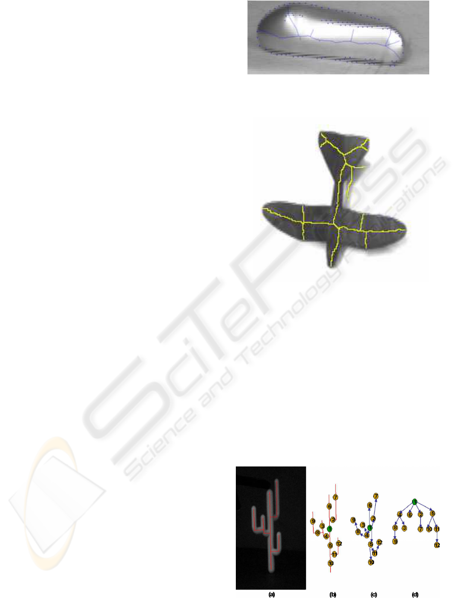
Figure 3: Hull object and 2D skeleton.

Figure 4: Plane object and 2D skeleton.

an off-line operation.

An on-line skeletonization of 2D scene image (sec-

ond line of ﬁgure 2) allows to build the 2D graph (line

3 of ﬁgure 2). Our method code these graphs in such

a way that each skeleton graph store topological and

geometrical information of the initial form. Indeed,

each node of the graph represents a skeleton element

that is a 2D segment for the 2D graph and a 3D seg-

ment for the 3D graph. Each edge in the graph rep-

resents a link between the different elements of the

skeleton (ﬁgure 5).

Figure 5: Graph construction from the skeleton.

ICINCO 2006 - ROBOTICS AND AUTOMATION

2.2 Matching

The recognition consists in establishing an isomor-

phism between the 3D graph from the database and

the 2D graph obtained from the image. The prob-

lem is to establish a good quality measure for graph

matching. In our application, this task is difﬁcult be-

cause the measure has to evaluate the similarity de-

gree between similar structures of two sub-graphs,

in order to manage the occlusion, shadow problems.

Therefore, it has to allow, in the recognition step, to

quickly choose the best model from the database (line

4 in ﬁgure 2) and also to perform a one to one node

matching, in order to locate and validate this hypoth-

esis (lines 5 to 12 in ﬁgure 2).

After studying several graph matching algorithms,

we implemented an isomorphism-based method us-

ing the topological signatures of each node. This

approach was used by Shokoufandeh (Shokoufandeh

and Dickinson, 1999), Siddiqi (Siddiqi et al., 1999)

and Macrini (Macrini et al., 2002) to match two shock

graphs. We introduced several modiﬁcations on this

method in order to obtain a robust matching algorithm

at the ﬁnal nodes level and also to carry out the nodes

”polygamy” i.e. a node can be matched at the same

time with several nodes.

In order to topologically describe a tree we used

graphs eigenspaces. We remember that each graph

can be represented as a adjacency matrix of {0, 1}.

The values 1 give adjacent nodes of the graph (and

0 on the diagonal). The eigenvalues (EV) of the adja-

cency matrix of the graph store some signiﬁcant struc-

tural properties of the graph (tree).

Explicitly, let T be a tree of maximum degree

∆ (T ) and T

, T

. . . , T

the sub-trees of its root. For

each sub-tree T

, the degree of its root is δ (T

). To

calculate this signature, we compute the eigenvalues

of each adjacency matrix of each sub-tree T

. Let S

be the sum of δ (T

) eigen values of T

. Then the

ordered elements S

, become the components of the

vector χ of dimension ∆ (T ) called topological sig-

nature and assigned to the tree’s root. If the elements

number S

is lower than ∆ (T ), then the vector is

ﬁlled with 0. This method is recursively repeated in

order to assign a vector to each node of the tree.

As we already mentioned, a trees isomorphism can

not exist between the image skeleton and the model

skeleton because of the occlusions or/and the noise.

The solution consists in ﬁnding a maximal cardinal-

ity and minimal weight matching in a bipartite graph

covering the nodes of the two skeletons. The bipartite

graph is a graph where each edge is pondered by the

topological distance.

We remember that our algorithm allows in a ﬁrst

time to index the object’s skeleton in a database -

which corresponds to the recognition step. In a sec-

ond time, it allow a one-by-one matching of the nodes

needed in the localization and veriﬁcation step.

2.3 Projection and Veriﬁcation

In the precedent step, due to the noise, there are sev-

eral matching hypothesis. To verify a hypothesis va-

lidity we will estimate the rigid transformation be-

tween the recognized (presumed) model and the cam-

era. The model projection on the image allows to ac-

cept or reject this hypothesis. Each matched couple

corresponds to a segment couple, one of the 2D skele-

ton and the other of the 3D curvilinear skeleton. We

project the primitives of the 3D object model on the

image plane. If the projected primitives do not co-

incide with the image primitives, according to a pre-

established threshold, then the hypothesis is rejected

and we treat the next hypothesis and so forth. If the

points of the 3D skeleton projected on the image do

not coincide with the points of the 2D skeleton, then

the object is not recognized.

This veriﬁcation module is based on the measure-

ment of this error (1) which is the distance in the

image (in pixels) between, each time, a 2D skeleton

point and a 3D skeleton point projected on the image.

error =

i=1



(ˆu

− u

)

+ (ˆv

− v

)



(1)

Where : N is the number of matching points,

, v

) the coordinates of a point image,

(ˆu

, ˆv

) estimation of the object’s point after

projection on the image plane.

The 3D pose estimation consists in ﬁnding the

rigid transformation (R, T ) minimising some calcu-

lated error (as the sum of error squares) of the one of

two collinearity equations (in the image space or in

the object space). The two methods generally used

to solve this problem are the Gauss-Newton and the

Levenberg-Marquardt methods (Lowe, 1991).

We used the method of Lu and al(Lu et al., 2000)

named Orthogonal Iteration (OI) algorithm. Contrary

to classical methods, used to solve the optimisation

problems on the whole, the OI algorithm cleverly ex-

ploits the speciﬁcal structure of the 3D pose estima-

tion problem.

To estimate the object’s pose, this algorithm uses

an appropriated error function deﬁned in the object’s

space. The error function is rewrited in order to accept

an iteration based on the classical solution of the 3D

pose estimation problem, called absolute orientation

problem.

This algorithm gives exact results and converges

quickly enough, therefore it is very interesting for

real-time applications.

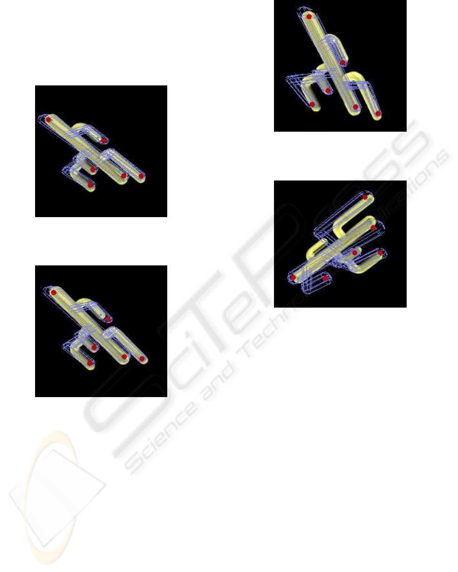
The ﬁgures 6 and 7 present some initialization re-

sults. On each ﬁgure, from left to right, there are the

TOWARD 3D FREE FORM OBJECT TRACKING USING SKELETON

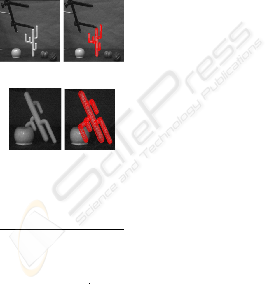
real object and the 3D model recognized by our algo-

rithm and superposed on the real image. There are 10

models in the database and the tests showed that our

methods can correctly recognize and localize several

3D objects even in presence of occlusions or auto-

occlusions and shadows (due to the strength of our

subgraph matching algorithm ).

Figure 6: Cactus object recognition among several objects.

Figure 7: Cactus object recognition with occlusion.

3 TRACKING

The initialization step coresponds to target pose com-

puting, without a priori knowledge of the scene. Once

the initial position of our object known, the tracking

process can start.

1. Tracking(ImageSequence{I

}):

{R, T} ←− InitialValues ;

while tracking not ﬁnished do

i ←− i + 1;

}←− 3DSkeletonEndpointsProjection;

}←− 2DSkeletonComputation( I

);

for each Endpoint e

of E

and e

of E

d ←− DistanceComputation(e

);

{(2D, 3D)} ←− CoupleChoice(d min);

10.

{R,T} ←− NewPoseComputation ({(2D, 3D)});

Figure 8: Tracking algorithm using skeletons.

The original position we used is the one calculated

on the ﬁrst image during the initialization step (line

2 of ﬁgure 8). The 3D skeleton is then projected on

the image plane, starting from this position, by using

the rotation and translation matrices calculated before

(line 5 of ﬁgure 8). The algorithm is based on the fact

that there are small movements between two video

frames. The positions of 2D skeleton points will be

very close from one frame to another.

We call p

the positions of the extremities j of the

2D skeleton in the frame i, numbered from 1 to n

(their number can vary with the frame). We call q

the positions of the projections on the image plane of

the 3D skeleton extremities, built using rotation and

translation matrices R and T respectively.

We suppose the initialization was correct, therefore

at the time of the projection of the 3D skeleton, the

points q

which were used to compute the position,

were near their matching points p

. In the next frame

(number (i + 1)), the points p

(i+1)j

are different from

points p

. Anyway, the deviation of the object be-

ing small, there is also a small variation for the 2D

skeleton position. This way the points q

which, by

construction, were very close to some points p

, will

be very close to some points p

(i+1)j

. The movement

of our object being very small, the old and the new

2D skeleton are very close one of the other, therefore

theirs extremities are also very close.

By measuring the pixel differences separating the

points p

(i+1)j

and q

, and sorting in ascending order,

we can form a number of pairs (p

(i+1)j

, q

). Whereas

during initialization matching between the extremities

of the 2D and 3D skeleton required heavy computing,

due to the fact that the position was unknown, it is al-

most immediate here by considering the points 3d at

the origin of q

(lines 6 to 9 in ﬁgure 8). The orthogo-

nal iteration algorithm we used for initialization is ap-

plied on the pairs (2DPoint , 3DPoint). The 3D points

being obtained by replacing q

by the original points

of the 3D skeleton. This provides us a new value for

R and T , which could be used in new computations

on the next frame (line 10 of ﬁgure 8).

We improved the Lowe method by integrating the

step of the graph matching in the tracking loop. For

example, in the case of an abrupt and irregular move-

ment or of an important occlusion, the model loses

the object. While applying, our algorithm of graph

matching we succeed to quickly re-localize this ob-

ject. We remind that in this step we already know

which 3D graph corresponds to the 2D graph, in

that case, it is sufﬁcient to make a one-to-one nodes

matching of two graphs. This step is very fast because

the skeletons graphs are small. This procedure is not

called during all the tracking process but only when

the projection error is greater then threshold. The al-

gorithm of the ﬁgure 8 becomes as the algorithm of

the ﬁgure 9.

ICINCO 2006 - ROBOTICS AND AUTOMATION

1. Tracking(ImageSequence{I

}):

{R, T} ←− InitialValues ;

while tracking not ﬁnished do

i ←− i + 1;

}←− 3DSkeletonEndpointsProjection;

}←− 2DSkeletonComputation( I

);

for each Endpoint e

of E

and e

of E

d ←− DistanceComputation(e

);

D ←− (d);

10.

if D > Threshold then

11.

{(2D, 3D)}←−1To1Matching(2DS,3DS);

12.

else

13.

{(2D, 3D)} ←− CoupleChoice(d min);

14.

{R,T}←−NewPoseComputation({(2D,3D)});

Figure 9: New tracking algorithm.

4 RESULTS OF SKELETON

TRACKING

Tracking was implemented in C++ in order to realise

real-time computing. There is a ﬁle in speciﬁc for-

mat allowing the passage from the initialization step,

realized in Matlab, to tracking. This ﬁle contains the

rotation and translation matrices corresponding to the

calculated position, as well as the model of the 3D

skeleton. The tests were realized on syntetic images

in order to validate our hypotesis. Using syntetic im-

ages allows to compare and estimate projection errors

more precisely, because we know the exact pose used

to generate our video. Moreover, that let us to gen-

erate various types of movement in various conﬁgu-

rations. Let us specify that although the used object

is a virtual one, its tracking in a sequence of frames

is made realistic (difﬁcult) by simulating shades, re-

ﬂections, noises, self-occlusions. The videos were

built with POV-Ray software to generate the images

and Virtual Dub to realize the video editing. To read

the video stream we used Intel’s OpenCV library.

Its main advantage is that it integrates some image

processing functions.

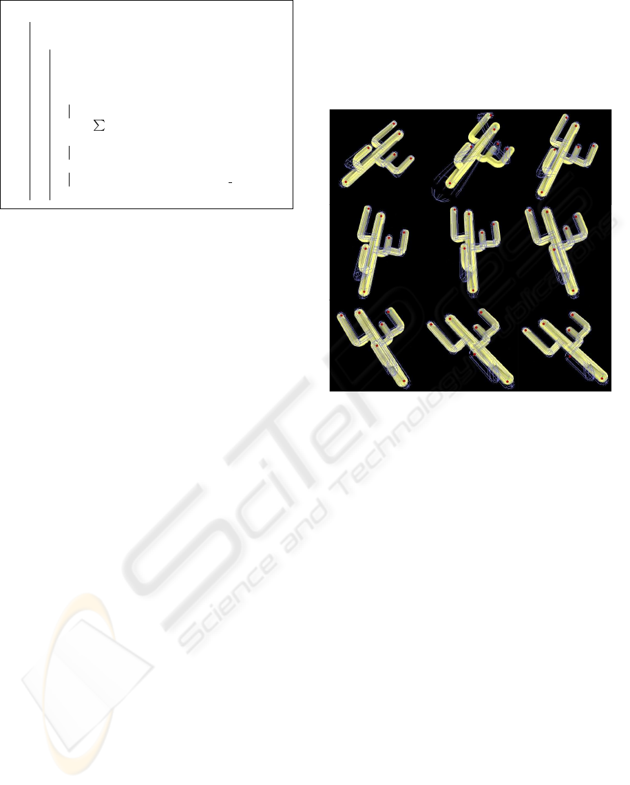
We did several tests and following we will present

only a part. The ﬁgure 10 shows the tracking result

on the cactus object, in a 68 ﬁrst frames sequence.

This ﬁgure represents, from left to right and from

up to down, the frames 1, 8, 16, 24, 32, 40, 48, 54,

67 respectively. We present here the most compli-

cated case. We simulated a complex movement with

a strong rotation around axis Z (optical axis of the

camera). The task becomes difﬁcult because of the

disappearance of a part of the object. The tracking

is carried out at the rate of 19 Hz by a wireframe

model (in magenta). The points of interests represen-

tating the extremities of the skeletons are red for the

3D points, and green for the 2D points. The graph

in the ﬁgure 11(a) represents the reconstruction errors

(in pixels) for this example. On the whole, the track-

ing is carried out correctly, it happens sometimes that

the model loose the object and recapture it in the next

sequence - image 2 of the ﬁgure 10 (frame 8) (due to

the integration of the graph matching procedure). We

can also observe this on the graph of the ﬁgure 11(a).

Figure 10: Object tracking sequence.

Another example is presented in the ﬁgure 11(b)

which represents the reconstruction errors of the ﬁrst

100 frames of a video (on a total of 2280 frames) in

which we simulated a translation following x and y

axes and a slight rotation following z. The ﬁgures 12,

13 and 14 represent the frames 27, 48 and 78 respec-

tively. We also notice that tracking is correct.

However, in some videos, the algorithm is not able

to efﬁciently track the object (ﬁgure 15). This is

essentialy owed to the absence of a sufﬁcient num-

ber of matchings occuring in the case of occlusions

or self-occlusions. The 3D pose parameters are not

correctly computed. We remember that the used or-

togonal iterations algorithm needs at least four good

non-coplanar matchings. However, after few frames

our algorithm recaptures the object and tracks it efﬁ-

ciently due to the integration of the graph matching

procedure.

5 CONCLUSION

In this article we presented a model based method for

3D free form object tracking. The results of adapt-

ing our skeleton recognition method to object track-

ing were encouraging and justify our approach. Nev-

ertheless we are conscient that some improvements

TOWARD 3D FREE FORM OBJECT TRACKING USING SKELETON

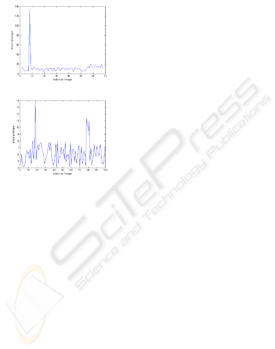
(a) During tracking in -R-

(b) During tracking in -RT-

Figure 11: Reconstruction error in pixels.

are needed for efﬁcient tracking. In our future works

we will focus on a 2D robust and fast skeletonization

method. We also project to compensate the weakness

of the Lowe method by adding a prediction step in our

algorithm.

REFERENCES

Attali, D. and Montanvert, A. (1997). Computing & sim-

plifying 2d & 3d continuous skeletons. In Computing

Vision and Image Understanding, Vol 3, N 67, pages

261–273.

Comport, A. I., Marchand, E., and Chaumette, F. (2003). A

real-time tracker for markerless augmented reality. In

Proceedings of the The 2nd IEEE and ACM Interna-

tional Symposium on Mixed and Augmented Reality,

pages 36–45.

Drummond, T. and Cipolla, R. (2002). Real-time visual

tracking of complex structures. In IEEE Transactions

on Pattern Analysis and Machine Intelligence vol. 24,

N. 7, pages 932–946.

Fabbri, R., Estozi, L., and da F. Costa, L. (2002). On

voronoi diagrams and medial axes. In Journal of

Mathematical Imaging and Vision, Vol 1, N 17, pages

27–40.

Gennery, D. B. (1982). Tracking known three-dimensionnal

objects. In Conf. American Association of Artiﬁcial

Intelligence, pages 13–17.

Gennery, D. B. (1992). Visual tracking of known three-

dimensionnal objects. In International Journal of

Computer Vision vol. 8, pages 243–270.

Harris, C. and Stennet, C. (1990). Rapid, a video rate object

tracker. In British Machine Vision Conference, pages

73–77.

Kegl, B. and Krzyzak, A. (2002). Piecewise linear skele-

tonization using principal curves. In IEEE Trans-

actions on Pattern Analysis and machine Intelli-

gence,vol. 1, N 24, pages 59–74.

Lowe, D. G. (1987). Three-dimensional object recognition

from single two-dimensional images. In Artiﬁcial In-

telligence, vol. 31, no. 3, pages 355–395.

Lowe, D. G. (1991). Fitting parametrized three-dimensional

models to images. In IEEE Transactions on Pattern

Analysis and Machine Intelligence, Vol 13, N 5, pages

441–450.

Lowe, D. G. (1992). Robust model-based motion tracking

through the integration of search and estimation. In

International Journal of Computer Vision vol. 8, no. 2,

pages 113–122.

Lu, C., Hager, G. D., and Mjolsness, E. (2000). Fast and

globally convergent pose estimation from video. In

IEEE Transactions on Pattern Analysis and Machine

Intelligence, Vol 22, N 6, pages 610–622.

Macrini, D., Shokoufandeh, A., Dickinson, S., Siddiqi, K.,

and Zucker, S. (2002). View-based 3-d object recog-

nition using shock graphs. In Proc. 16 Th Internatonal

Conference on Pattern Recognition, Quebec.

Malandain, G. and Fernandez-Vidal, S. (1998). Euclidean

skeletons. In Image and Vision Computing, vol. 16,

pages 317–327.

Marchand, E., Bouthemy, P., Chaumette, F., and Moreau, V.

(1999). Robust real-time visual tracking using a 2d-3d

model-based approach. In International Conference

on Computer Vision vol. 1, pages 262–268, Greece.

Nilsson, F. and Danielsson, P. (1997). Finding the minimal

set of maximum disks for binary objects. In Graphical

Models and Image Processing, N 59, vol. 1, pages 55–

60.

Shokoufandeh, A. and Dickinson, S. (1999). Applications

of bipartite matching to problems in object recogni-

tion. In Pro., ICCV Workshop on Graph Algorithms

and Computer Vision.

Siddiqi, K., Shokoufandeh, A., Dickinson, S. J., and

Zucker, S. (1999). Shock graphs and shape matching.

In International Journal of Computer Vision, Vol 35,

N 1, pages 13–32.

Skrypnyk, I. and Lowe, D. (2004). Scene modelling, recog-

nition and tracking with invariant image features. In

Proceedings of the The 3rd IEEE and ACM Interna-

tional Symposium on Mixed and Augmented Reality,

pages 110–117, Arlington,VA.

ICINCO 2006 - ROBOTICS AND AUTOMATION

Tek, H. and Kimia, B. (1998). Curve evolution, wave prop-

agation and mathematical morphology. In fourth In-

ternational Symposium on mathematical Morphology.

Vacchetti, L., Lepetit, V., and Fua, P. (2004). Stable real-

time 3d tracking using online and ofﬂine informa-

tion. In IEEE Transaction on Pattern Analysis and

Machine, vol. 26, N 10, pages 1385–1391.

Figure 12: Frame 27.

Figure 13: Frame 48.

Figure 14: Frame 78.

Figure 15: Incorrect tracking.

TOWARD 3D FREE FORM OBJECT TRACKING USING SKELETON