
FUZZY CLASSIFICATION BY MULTI-LAYER AVERAGING
An Application in Speech Recognition
Milad Alemzadeh, Saeed Bagheri Shouraki, Ramin Halavati
Computer Engineering Department, Sharif University of Technology, Tehran, Iran
Keywords: Speech Recognition, Fuzzy Number, Multi-Layer Averaging.
Abstract: This paper intends to introduce a simple fast space-efficient linear method for a general pattern recognition
problem. The presented algorithm can find the closest match for a given sample within a number of samples
which has already been introduced to the system. The fact of using averaging and fuzzy numbers in this
method encourages that it may be a noise resistant recognition process. As a test bed, a problem of
recognition of spoken words has been set forth to this algorithm. Test data contain clean and noisy samples
and results have been compared to that of a widely used speech recognition method, HMM.
1 INTRODUCTION
Pattern recognition is one of the oldest challenges of
researchers in different areas such as artificial
intelligence, interactive graphic computers and
computer aided design. Different kinds of
recognition can also be generalized as a pattern
recognition problem. A pattern is an arrangement of
descriptors. Therefore a wide range of problems can
easily be seen as a pattern recognition problem.
Considering this general view, this paper tries to
demonstrate a time and space efficient yet simple
approach for a pattern matching problem.
The presented algorithm can compare a given
sample to a number of samples in its database and
specify the closeness of each sample of database to
the given one. This comparison can be served to find
the closest match which can be interpreted as a
recognition process. The samples used in this
algorithm are generally N-dimensional arrays, but
since 2D arrays are mostly the case (images,
spectrograms and etc.) in pattern recognition
processes, the algorithm has been developed based
on such structure. The details about this issue have
been discussed in next section.
For displaying the effectiveness of presented
method and also for demonstrating its ability to
solve practical problems, this algorithm has been
applied to a speech recognition problem and tested
and compared with one of the best methods of this
category, Hidden Markov Model. The flexibility of
this method to noise which is one the most important
concepts of speech recognition has also been tested.
The next section explains the details of the
problem in hand and how the discussed general
domain has been mapped to a speech recognition
issue. In section 3, the steps of recognition process is
explored in which the idea of Multi-Layer Averaging
(MLA) combined with fuzzy classification is
described. The complexity of the algorithm is then
calculated and shown in section 4 which shows its
time and space efficiency. Finally, the results and
comparisons are presented in section 5.
2 PROBLEM SPACE
As it was mentioned, a pattern recognition problem
can be a general concept. This section tries to limit
the definition of the problem although it can easily
be extended to more complex forms. First, a general
view is established to display how this method can
be applied to different areas. Then an application of
this definition in recognition of a spoken word signal
will be presented.
122
Alemzadeh M., Bagheri Shouraki S. and Halavati R. (2006).
FUZZY CLASSIFICATION BY MULTI-LAYER AVERAGING - An Application in Speech Recognition.
In Proceedings of the Third International Conference on Informatics in Control, Automation and Robotics, pages 122-126
DOI: 10.5220/0001206001220126
Copyright
c
SciTePress
2.1 General View
The idea of MLA can be applied on any arrangement
of numeric data with subtle adaptations. The
structure used in this paper is a 2-Dimentional
matrix of integer numbers. The goal is to find a
match for a given sample among a number of
samples which has already been introduced and
analyzed by the system.
Definition: A Sample is a matrix of size (m × n)
of integer numbers.
Different samples do not necessary have the
same size. However it is needed for further steps of
algorithm to reduce sample data to a specified size
for all samples. This reduction is done by
quantization process.
Quantization process is a process which takes
raw data from input source and converts these data
to integer values in the form of a matrix with a
predefined size. First part of quantization is
converting the numbers to integer values. This can
be done by a function to map the input range to a
desired range so that a proper distribution of
numbers is achieved.
In second part, to resize the dimensions of input
data, a grid of specific size is assumed upon current
data and the numbers of each block of the grid are
averaged and the result will represent the value of
that block. The above view has been applied to a
specified case of speech recognition which is
described in the following sub-section.
2.2 Word Recognition Problem
Speech recognition can be divided to smaller
problems. The range of these problems can differ
from recognition of phoneme to a word then a
sentence and ultimately continuous speech. The
number of speakers is also an important factor. This
paper deals with the recognition of spoken words of
a single speaker. The goal is to get a new sample (a
spoken word in this case) from a speaker and
classify it within a number of existing samples
which are already acquired from the same speaker.
There are two technical assumptions considered
in implementation of this algorithm. First
assumption is that words are pronounced normally
i.e. the relative lengths of phonemes of a word are
almost equal for different pronunciations of the same
word. Second assumption is that each sample is
properly clipped i.e. there are no blank or irrelevant
data in the beginning and end of a sample.
Before the recognition process can be applied, it
is needed for both train and test data to be converted
to the format discussed in previous sub-section. To
do so, spectrogram of each sample is calculated.
Spectrogram is simply amplitudes of a range of
frequencies in small time slices over speech signal
time period.
After acquiring spectrograms of each sample, a
normalization algorithm makes sure that data are
converted to integer and uniformly distributed over
the range of [0, 255]. The result is a matrix of
integer numbers which its sizes are dependant of
both length of time of the word and the size of FFT
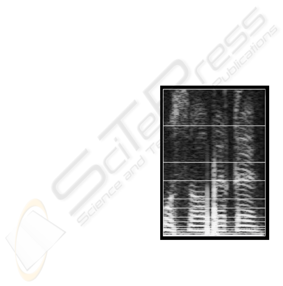
algorithm (256, 512, etc). Figure 1 shows a
spectrogram of a spoken word. The horizontal axis is
time and the vertical axis is frequency.
Figure 1: Spectrogram of a word.
The last step of this preprocess is averaging data
of spectrograms so that all samples have equal sizes.
For this reason, the spectrogram is divided to 12
frequency bands and 32 time bands. It is notable that
the number of time bands should be in form of a
power of 2. The reason will be explained in next
section. The lengths of all time bands are equal.
However the length of frequency bands differs.
FUZZY CLASSIFICATION BY MULTI-LAYER AVERAGING - An Application in Speech Recognition
123
Because lower frequencies contain more information
than higher ones, the length of bands increases for
higher frequencies. The horizontal lines displayed in
figure 1 separate frequency bands.
Intersection of a frequency band and a time band
creates a block. After averaging the data of each
block, a matrix of (32 × 12) is achieved for each
sample. These matrices are fit to be dealt by
recognition process. The idea of averaging is used
for correcting probable noises and displacements. In
the next section, the MLA algorithm is used to
recognize test samples which are also converted to
matrices of above size and format.
3 RECOGNITION PROCESS
The main idea of MLA for matching a sample within
a group is to eventually eliminate non-similar
samples by giving them a penalty so that the best
match which is the most similar sample remains
with least penalty. In order to accomplish this goal,
the following fact is used: if two series of numbers
are almost similar their averages are also similar. In
other words, if averages of two series of numbers are
not similar, those series are not similar either
(however the reverse is not true). Therefore this
dissimilarity can be used to eliminate samples.
3.1 Multi-Layer Averaging
Using the idea introduced above, MLA tries to
iteratively give penalty points to samples by
comparing their averages. The comparison is done in
different layers. The following steps explain the
algorithms. The sample to be recognized is called
"Test Sample" and the sample from database of
system upon which test sample is checked is called
"Matching Sample"
Step 1: Choose a matching sample from
database. Set its penalty point to zero.
Step 2: Set the number of averages (N
a
) in first
layer to 1. Each of two samples should have C
members which should be a power of 2.
Step 3: Define variable M as C / N
a
. Average
every M members of both test and matching samples
which results in N
a
numbers for each samples. Call
them A
i
and B
i
for which
a
Ni ≤
≤
1 .
Step 4: Compare each average of test sample (A
i
)
to its corresponding average in matching sample
(B
i
). Add a penalty point to the points of matching
sample according to comparison method.
Step 5: Multiply N
a
by 2 for next layer. If N
a
is
not larger than C go to step 3.
Step 6: If there are any remaining sample in
database go to step 1. Otherwise, sort matching
samples ascending based on their penalty points.
Return first sample in the list as answer.
The penalty point in step 4 can be defined
differently to achieve better results. It can simply be
average of all of differences of each A
i
and B
i
:
() ()
∑
=
=
−=−=
a
a
N
i
ii
a
ii
N
i
BA
N
BAPenalty
Avg
1
1
1
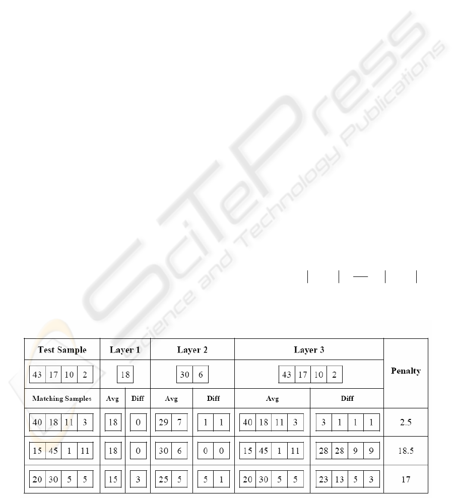
Figure 2: MLA algorithm using simple differential penalty point strategy.
ICINCO 2006 - SIGNAL PROCESSING, SYSTEMS MODELING AND CONTROL
124
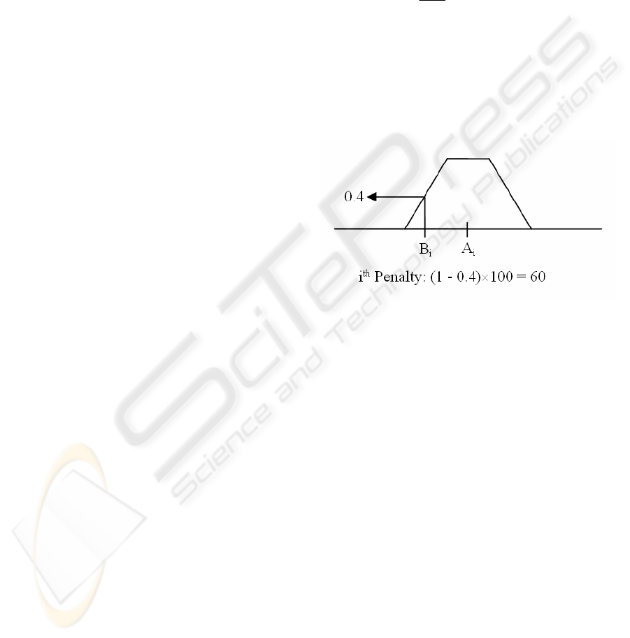
Figure 2 shows an illustration of above algorithm
with such penalty point strategy for a test sample
and 3 matching samples having 4 members which in
fact is the number of time bands for speech
recognition problem. Only 1 frequency band is
considered just for the ease of understanding. This
means that our samples in this example are matrices
of (4 × 1).
First matching sample in figure 2 is most similar
one and gets the least penalty. Although second
matching sample gets no penalty in first two layers
but it gets largest penalty in last level. It should be
mentioned again that differences of each layer are
averaged and sum of these averages will be the
penalty point. For better understanding, let us review
how the penalty of third matching sample is
calculated.
In first layer, the average of all members (20, 30,
5, and 5) is 15 and the difference of this value with
its correspondence in test sample (18) is equal to 3
which is added to penalty points of this matching
sample (P = 3). Then in second layer, average of
first two members (20 and 30) is 25 and average of
second two members (5 and 5) is 5. The differences
of these averages with their correspondence (30 and
6) are respectively 5 and 1. The penalty point of this
layer is then average of 5 and 1 which is 3 and adds
to overall penalty (P = 3+3 = 6). In last layer, each
member acts as an average and therefore the
differences with the corresponding values of test
sample are 23, 13, 5 and 3. The penalty point of this
layer is average of these values which equals to 11.
Finally the overall penalty is P = 6 + 11 = 17. All of
these calculations were based on differential penalty
point strategy. A fuzzy penalty point strategy is
presented in next sub-section.
3.2 Fuzzy Classification
The chosen penalty point strategy in above
algorithm is the strategy to eliminate non-similar
samples so that the best match gets the least penalty.
Therefore, it can be considered as a classifier. One
simple method has been introduced in previous sub-
section. Another strategy is used in this project
which is based on fuzzy numbers.
Instead of calculating the difference between A
i
and B
i
, the averages of test sample (A
i
) are
considered fuzzy numbers. These fuzzy numbers are
defined by a symmetrical trapezoidal membership
function (the size of this trapezoid depends on the
nature of the problem and will be specified mostly
by trail and error to achieve best results). Then,
membership values of the corresponding averages of
matching sample (B
i
) are calculated. The overall
penalty for all pairs of averages is calculated by:
(
)
(
)
()
∑
=
=
−=
×−=
a
i
i
a
N
i
i
A
a
i
A
N
i
B
N
BPenalty
Avg
1
~
~
1
)(1
100
100)(1
μ
μ
If each two averages are close enough, the
membership value would be 1 and then the penalty
is 0. Otherwise it gets a linear penalty up to 100.
Figure 3 shows a fuzzy number (A
i
) and how a
penalty is given to a corresponding average (B
i
).
Figure 3: Fuzzy number and penalty calculation.
In order to apply the MLA algorithm to the
presented problem in previous section, a sample is
treated like 12 sub-samples for every frequency band
and each of these 12 sub-samples are given to the
algorithm and a penalty point is gathered for each
band and these penalty points are added up to one
penalty point for the whole sample.
4 COMPLEXITY OF
ALGORITHM
It is very easy to show that both space and time
complexity of MLA algorithm is Ω(n) in which n is
the number of trained samples. The samples which
are introduced to the system are usually called
trained samples. However it should be considered
that there is no training stage in this algorithm.
Adding new samples only involves calculating
spectrogram with FFT algorithm which can be done
very fast, normalizing which is applying a function
to each value of spectrogram and finally averaging
FUZZY CLASSIFICATION BY MULTI-LAYER AVERAGING - An Application in Speech Recognition
125
spectrogram to acquire a matrix of (32 × 12) and
saving this matrix for further use.
The memory space needed for this algorithm is
32×12 integer numbers for each sample. Considering
the range of these integers [0, 255], only 1 byte is
needed for each number. Therefore each sample
takes 384 bytes and the growth of space is 384×n
hence Ω(n).
Time complexity for this algorithm can be
calculated by considering the comparisons for each
sample. The number of layers is always constant (6
layers in this case: 2
0
to 2
5
). In presented problem
there are 12 frequency bands which are also
constant. Therefore number of comparisons for each
sample is constant and same for all samples. This
shows that the complexity is again Ω(n). However,
the sorting step takes about O(n Log n). This causes
the time complexity to be O(n Log n) in overall
which is still acceptable as a fast algorithm.
The small size of memory needed for each
sample and the speed of recognition of a word make
this algorithm very suitable for voice commands in
mobile devices such as cell phones, PDAs and etc.
Since there are only one or two words for each
command and considering the results in next section,
this simple algorithm seems very efficient and useful
for the purpose of voice command.
5 RESULTS
The presented algorithm has been implemented and
tested for a single speaker with 100 words. The
results have been compared to that of a widely used
method in speech recognition, HMM. In order to
measure flexibility of this algorithm to noise,
different kinds of noises are applied to test data.
Table 1 shows these results.
For this purpose, a database of samples is
generated which contains about 8 different
pronunciations of a same word, for 100 words which
add up to 800 samples. All samples were introduced
to system except one for each word. Then these
unused samples were tested by system and asked for
recognition. The entry called "Clean" in table 1
refers to these results.
Afterwards, different amounts of two kinds of
noises, White Noise and Babble Noise, are added to
test data and asked again to be recognized. Other
entries of table 1 show these results. Also, "First
Answer" means first recognized answer is the
correct answer and "Third Answer" means one of the
first three answers is the correct answer. The same
data has been tested with HMM approach and its
results are also included for comparison.
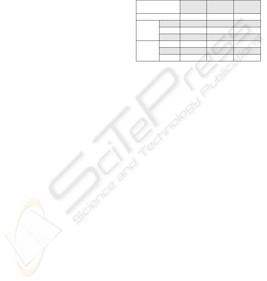
Table 1: Experimental results.
HMM
First
Answer
Third
Answer
Clean 100 % 98 % 99 %
20 db 99 % 91 % 96 %
10 db 74 % 90 % 96 %
White
Noise
0 db 4 % 84 % 91 %
20 db 98 % 98 % 99 %
10 db 92 % 92 % 95 %
Babble
Noise
0 db 39 % 44 % 72 %
Table 1 shows that while the efficiency of HMM
algorithm drops down sharply with noisy data, the
presented algorithm keeps its efficiency even with
intensive noise. Also, it can be noted that because of
the smoothing property of averaging, this algorithm
has a good resistance to white noise and this can be
concluded from above results. However, because the
babble noise destroys the information of lower
frequencies, it can affect the efficiency of this
algorithm. Therefore, the first 3 lower frequency
bands of spectrograms have been ignored to achieve
better results in table 1.
REFERENCES
Zimmermann, H.J., 1996. Fuzzy set theory and its
applications, Kluwer Academic Publishers.
Boston/Dordrecht/London, 3
rd
edition.
Gonzalez, R., Woods, R., 2001. Digital image Processing,
Prentice Hall. New Jersey, 2
nd
edition.
Halavati, R., Bagheri, S., Sameti, H., Babaali, B., 2005. A
novel noise immune fuzzy approach to speech
recognition. In International Fuzzy Systems
Association 11th World Congress. Beijing, China.
Babaali, B., Sameti, H., 2004. The sharif speaker-
independent large vocabulary speech recognition
system. In The 2nd Workshop on Information
Technology & Its Disciplines (WITID 2004). Kish
Island, Iran.
Duchateau, J., Demuynck, K., Compernolle, D.V., 1998.
Fast and Accurate Acoustic Modelling with Semi-
Continuous HMMs. In Speech Communication,
volume 24, No. 1, pages 5--17.
Ohkawa, Y., Yoshida, A., Suzuki, M., Ito, A., Makino, S.,
2003. An optimized multi-duration HMM for
spontaneous speech recognition. In EUROSPEECH-
2003. 485-488.
ICINCO 2006 - SIGNAL PROCESSING, SYSTEMS MODELING AND CONTROL
126
