
SMOOTH TRAJECTORY PLANNING FOR FULLY
AUTOMATED PASSENGERS VEHICLES
Spline and Clothoid based Methods and its Simulation
Larissa Labakhua
University of Algarve
Escola Superior de Tecnologia/ADEE, Faro, Portugal
Urbano Nunes, Rui Rodrigues and Fátima S. Leite
Institute of Systems and Robotics, University of Coimbra
Coimbra, Portugal
Keywords: Trajectory planning, splines, clothoids, trajectory tracking, fully-automated vehicles, passenger comfort.
Abstract: A new approach for mobility, providing an alternative to the private passenger car, by offering the same
flexibility but with much less nuisances, is emerging, based on fully automated electric vehicles. A fleet of
such vehicles might be an important element in a novel individual, door-to-door, transportation system to
the city of tomorrow. For fully automated operation, trajectory planning methods that produce smooth
trajectories, with low associated accelerations and jerk, for providing passenger´s comfort, are required.
This paper addresses this problem proposing an approach that consists of introducing a velocity planning
stage to generate adequate time sequences for usage in the interpolating curve planners. Moreover, the
generated speed profile can be merged into the trajectory for usage in trajectory-tracking tasks like it is
described in this paper, or it can be used separately (from the generated 2D curve) for usage in path-
following tasks. Three trajectory planning methods, aided by the speed profile planning, are analysed from
the point of view of passengers' comfort, implementation easiness, and trajectory tracking.
1 INTRODUCTION
Negative side effects of car use in build-up areas
jeopardise the quality of life. Technology driven
inventions like cybernetic transport systems may
contribute to sustainable urban mobility. In this
context, a new approach for mobility providing an
alternative to the private passenger car, by offering
the same flexibility but with much less nuisances, is
emerging, based on fully automated electric
vehicles, named cybercars (Parent 2003; Cybercars
2001). A fleet of such vehicles might be an
important element in a novel individual, door-to-
door, transportation system to the city of tomorrow.
These vehicles must be user-friendly, easy to handle
and safe, not only for passengers but also for the
other road users. These vehicles are already in
operation in specific environments featuring short
trips at low speed (Parent 2003; Bishop 2005).
For fully automated operation, trajectory
pl
anning methods that produce smooth trajectories,
with low associated accelerations and jerk, are
required. Although motion planning of mobile
robots has been thoroughly studied in the last
decades, the requisite of producing trajectories with
minimum accelerations and jerk (integrating both
lateral and longitudinal accelerations) has not been
traceable in the technical literature. A global
minimum-jerk trajectory planning approach is
proposed in (Piazzi 2000) but in the context of joint
space trajectories of robot manipulators.
This paper addresses the problem of generating
sm
ooth trajectories with low associated
accelerations, proposing an approach that consists of
introducing a velocity planning stage to generate
adequate time sequences to be fed into the
interpolating curve planners. The generated speed
profile can be merged into the trajectory for usage in
trajectory-tracking tasks like it is described in this
89
Labakhua L., Nunes U., Rodrigues R. and S. Leite F. (2006).
SMOOTH TRAJECTORY PLANNING FOR FULLY AUTOMATED PASSENGERS VEHICLES - Spline and Clothoid based Methods and its Simulation.
In Proceedings of the Third International Conference on Informatics in Control, Automation and Robotics, pages 89-96
DOI: 10.5220/0001205700890096
Copyright
c
SciTePress
paper, or it can be used separately (from the
generated 2D curve) for usage in path-following
tasks (Solea 2006). Three trajectory planning
methods used to generate smooth trajectories from a
set of waypoints, embedding a given speed profile,
are analysed from the point of view of passengers'
comfort, easiness of implementation, and trajectory
tracking performance. The trajectory-planning
methods studied are the following ones: cubic spline
interpolation, trigonometric spline interpolation, and
a combination of clothoids, circles and straight lines.
For its evaluation, the well-known Kanayama
trajectory-tracking controller was used (Kanayama
1991). The kinematics model of a Robucar vehicle
(platform used in our autonomous navigation
experiments) is used to evalute through simulations
the studied trajectory planning methods.
2 ACCELERATION EFFECTS ON
THE HUMAN BODY
For a vehicle following a trajectory at speed ,
accelerations are induced on the passengers, which
can be expressed as
v
T
dv dv d
aev
dt dt dt
θ
== +
N
e
(1)
where denotes the longitudinal velocity (tangent
to the trajectory),
v
θ
is the vehicle orientation, and
and are unit vectors in the tangent and
normal trajectory directions, respectively. Moreover
T
e
N
e
1d
v
dt
θ
ρ
=
(2)
where
ρ
is the curvature radius. From (1) and (2)
one gets the longitudinal acceleration (tangential
component), induced by variations in speed,
T
dv
a
dt
=
(3)
and lateral accelerations (normal component),
originated by changes in vehicle´s orientation,
whose values are also affected by the vehicle speed:
2
1
L
d
av
dt
θ
v
ρ
==
(4)
The lateral acceleration is function of the trajectory
curvature and speed (see (4)). Assuming constant
speed, the smaller is the curvature the smaller is the
induced lateral acceleration, and therefore less
harmful effects on the passengers. The ISO 2631-1
standard (Table 1) relates comfort with the overall
r.m.s. acceleration, acting on the human body,
defined as
22 22 22
wxwxywyzw
akakaka=++
z
(5)
where , , , are the r.m.s. accelerations on
wx
a
wy
a
wz
a
,,
x
yz
axes respectively, and
, , ,
x
yz
kkk
are
multiplying factors. For a seated person
1.4, 1
xy z
kk k
=
==
. For motion on the
x
y
-plane,
0
wz
a
=
. The local coordinate system is chosen so
that its
x
-axis is aligned with the longitudinal axis
of the vehicle, and it’s - axis defines the trajectory
lateral direction.
y
2.1 Speed Profile
Trajectory planning for passenger's transport
vehicles must generate smooth trajectories with low
associated accelerations and jerk. As expressed by
(3) and (4), lateral and longitudinal accelerations
depend on the vehicle´s speed. Thus, the trajectory
planner should not only generate a smooth curve
(spatial dimension) but also its associated speed
profile (temporal dimension).
Table 1: ISO 2631-1 Standard.
Overall Acceleration Consequence
2
0.315 /
w
am< s
Not uncomfortable
2
0.315 0.63 /
w
am<< s
A little uncomfortable
2
0.5 1 /
w
ams<<
Fairy uncomfortable
2
0.8 1.6 /
w
am<< s
Uncomfortable
2
1.25 2.5 /
w
am<< s
Very uncomfortable
2
2.5 /
w
am> s
Extremely uncomfortable
Using Table 1 and equation (5), for "not
uncomfortable" accelerations, the longitudinal and
lateral r.m.s. accelerations must be less than
. Speed profiles can be calculed under this
constraint, and consequently appropriate time-
interval values sequences obtained to be used by the
curve planners. Assuming a constant speed and a
perfect arc cornering with a radius , the reference
speed in corners (segment between waypoints
i and
) is
2
0.21 /ms
r
j
2
, 0.21 /
ij T T
vara ms
≤
⋅≤
(6)
It makes sense to consider a straight course
segment just before each corner for reducing speed,
and others after corners for increasing speed. So, the
reference speed on the straight segments begin
(end), designated by the waypoint , can be
calculated as
k
2
, 0.21 /
kiL L
vvat a ms=±Δ ≤
(7)
ICINCO 2006 - ROBOTICS AND AUTOMATION
90
2/
L
tlaΔ=
(8)
where the waypoint i designates the corner begin
(end), and is the straight segment length.
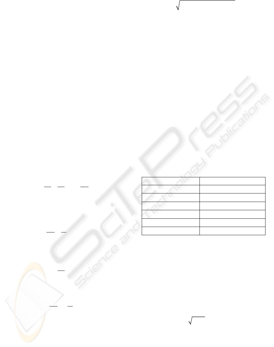
Figure 1 shows an urban road way with very
close corners, a roundabout, and a set of waypoints
defined by stars.
1 2
3
4
5
6
7
89
10
11
12
13
14
15
16
17
18
19
20
21
2223
24
25
26
28 m
18 m
R 11 m
34 m
18 m
27 m
Figure 1: Urban road way with very close corners, a
roundabout, and waypoints defined by stars.
0
0,2
0,4
0,6
0,8
1
1,2
1,4
1,6
1,8
1234567891011121314151617181920212223242526
Waypoints
Reference Velocity (m/s)
12
43
87
5
6109
11
1817
12
1615
13 14
2019
2423
21 22 2625
Figure 2: Speed profile defined by speed values at the
waypoints specified in Fig.1: .
,1,2,,26
ri
vi=
For the purpose of comparison of the three trajectory
planning algorithms, applied to the scenario depicted
in Fig.1, and somehow to observe the above
acceleration constraints, it was empirically defined
the speed profile shown in Fig.2. A simple algorithm
to generate a speed profile curve using a second
order polynomial is presented in (Solea 2006),
which is a step in an iterative trajectory planning
method that generates smooth curves with bounded
associated accelerations.
1
C
3 KINEMATICS MODEL
Cybercars are expected to be used in urban areas,
airport terminals, pedestrian zones, etc, i.e. in places
where the vehicle will move at relatively low speed.
Therefore, kinematics-based trajectory control can
be considered. These vehicles are under-actuated
systems, with two controls, speed and steering angle,
but evolving in a
3
D
configuration space
{}
,,xy
θ
,
the first 2 coordinates for the
2
D
position and the
−κ
−
κ
δ
TD
δ
TE
δ
FE
δ
FD
ρ
F
ρ
T
G
x
x
T
y
T
y
θ
V
T
V
F
T
F
A
B
C
D
e
L
H
ρ
FD
ρ
FE
α
α
β
β
ρ
TD
ρ
TE
ϕ
ϕ
ϕ
ϕ
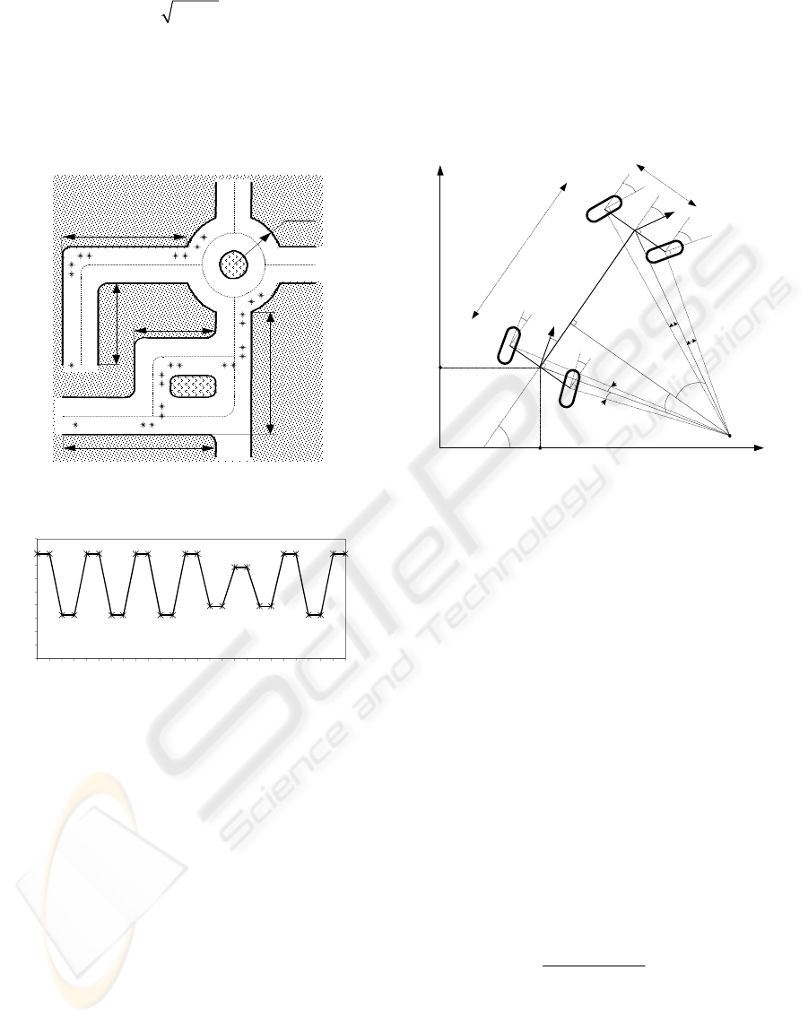
Figure 3: Kinematics model of a 4-wheel car-like vehicle
with front and rear steering capability.
third for the vehicle orientation. A representation of
the kinematics model of Robucar (bi-steerable, 4-
wheels actuated vehicle manufactured by Robosoft)
is shown in Fig. 3. The model shows the possibility
to steer both the rear and front pairs of wheels. The
rear steering angle is proportional by a factor -k to
the front steering angle. If the angle ϕ represents the
front wheels' steering command, the back wheels
will be deflected from the central axis of the vehicle
by an angle -kϕ. Assuming that the wheels roll
without slipping, the rear and front steering angles
give the directions of the velocities at points F and
T, respectively. Hence, the position of the
instantaneous turning centre of the solid, point G in
Fig.3 can be deduced. Using the geometrical model
of Fig. 3, the kinematics model of the vehicle¸ with
the possibility of steering both the rear and front
wheels, can be derived (Sekhavat 2000):
2
cos( )
0
sin( )
0
sin( )
0
cos( )
1
0
0
F
T
F
T
FF
T
F
F
T
k
x
k
y
k
qv
L
k
θϕ
θϕ
ϕϕ
θ
ϕ
ϕ
ϕ
−
⎡⎤
⎡⎤
⎡⎤
−
⎢⎥
⎢⎥
⎢⎥
⎢⎥
+
⎢⎥
⎢⎥
v
=
=⋅+
⎢⎥
⋅
⎢⎥
⎢⎥
⎢⎥
⎢⎥
⎢⎥
−
⎢⎥
⎣⎦
⎣⎦
⎣⎦
⋅ (9)
where L is the vehicle length and v
2
defines the front
wheels steering angular speed. The rear wheels
steering angular speed is .
2
kv
SMOOTH TRAJECTORY PLANNING FOR FULLY AUTOMATED PASSENGERS VEHICLES - Spline and Clothoid
based Methods and its Simulation
91
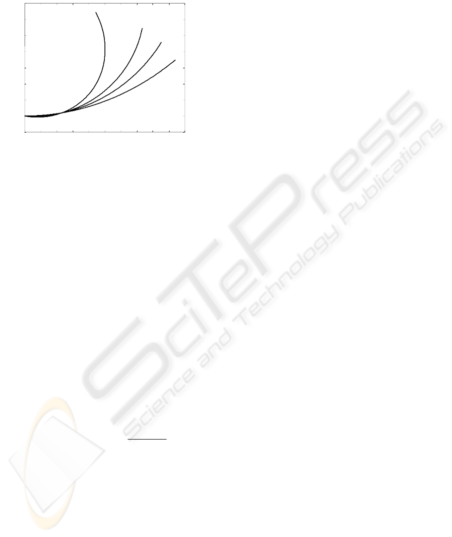
The results shown in Fig. 4 were calculated using
model (9). For a given front steering angle
ϕ
, the
effect of the rear steering angle is shown.
0 2 4 6 8 10 12 14 16 18 20
-2
0
2
4
6
8
10
12
14
X [m]
Y [m]
k=0
k=0.5
k=1
k=2
Steering angle
ϕ
F
= 5º
Figure 4: Car-like vehicle trajectories, using the same
front wheel steering angle
5º
F
ϕ
=
and different values of
the rear steering angle, given by the coefficient k.
Autonomous vehicles are expected to be used in
places such as city centres with narrow areas and
wherever it is needed to share the space with
pedestrians. So, it is also important to know the
position of each wheel, in order to avoid any kind of
casualties, sidewalks, etc. Solving the kinematics
model (9), and knowing the vehicle length L and its
width e, it is possible to derive an output equation
for the wheels' positions.
4 TRAJECTORY PLANNING
METHODS
4.1 Cubic Splines
We assume that is a chosen partition
of the time interval
[
01 m
tt t<< <
]
0
,
m
tt
, and that
are given distinct points in
01
,,,
m
pp p…
()
2
!
!!
n
rnr
ℜ
−
. We are
interested in the construction of a smooth curve in
2
ℜ
which goes through the point at time , for
all with prescribed initial and final
velocities ( and respectively). The instants of
time are chosen in order that the trajectory satisfies a
reasonable criterion of performance. Typically, this
interpolation problem can be solved by a cubic
spline, which is roughly a smooth concatenation of
simple cubic polynomial curves. More precisely, a
curve
,
k
p
k
t
0,1, , ,k= … m
0
v
m
v
()St
[
]
0
,
m
ttt∈
, is a cubic spline in
2
ℜ
if it
fulfils simultaneously the following:
1) is defined in each subinterval
[
()St
]
1
,
kk
tt
+
by:
(10)
23
11 1 1
2
22 2 2
()
kk k k
k
kk k k
abtctdt
St
abtctdt
⎛⎞
++ +
=
⎜⎟
++ +
⎝⎠
3
2) is
()St
2
C
−
smooth in
[
]
0
,
m
tt
, i.e., ,
()St
(),St
′
()St
′
′
are continuous functions in
[
]
0
,
m
tt
;
3)
()
kk
St p
=
,
0, ,km
=
…
,(interpolation conditions);
4)
0
()St v
0
′
=
and (boundary
conditions).
()
m
St v
′
=
m
All the coefficients in (10) are uniquely
determined by solving a set of linear algebraic
equations arising from conditions 2), 3) and 4). The
cubic spline
is a smooth concatenation of each
spline segment and thus uniquely computed
(Gerald et al., 1984).
()St
()
k
St
4.2 Trigonometric Splines
An alternative to build a –smooth trajectory in a
two-dimensional environment satisfying all the
requirements at the beginning of this section is based
on the construction of a trigonometric interpolating
curve, described in (Nagy 2000), (Rodrigues 2003).
This curve is again obtained by putting together
smaller pieces (spline segments). However, one
particular but important feature of this construction
is that each piece can be computed separately. As a
consequence, one may reduce the computations of
each spline segment to the time interval
[
2
C
]
0,1
, thus
simplifying notations.
The piece connecting point (at ) to
point
k
p
0t =
1k
p
+
(at
1t
=
) is denoted by and given
by the following convex combination of two other
curves,
()
k
St
()
k
L
t
and :
()
k
Rt
22
() cos ( /2) () sin ( /2) ().
kk
St t Lt t Rt
ππ
=+
k
The curves
k
L
and are called respectively the
left component and the right component of the spline
segment and will be computed from the local data as
follows. The name “trigonometric spline” is
suggested by the expression which defines the spline
components.
k
R
• Computation of
k
L
( ):
0k ≠
If the points ,
k
p
1k
p
+
and define a straight
line, then is the line segment connecting
1k
p
−
()
k
Lt
k
p
ICINCO 2006 - ROBOTICS AND AUTOMATION
92
(at ) to (at ). Otherwise, consider the
circle defined by the 3 points and let
0t =
1k
p
+
1t =
()
k
L
t
be the
circular arc joining (at ) and (at
) that does not contain .
k
p
0t =
1+k
p
1=t
1k
p
−
• Computation of ( ):
k
R km≠
The previous algorithm (for the left component)
is also implemented to compute the right component,
but uses instead the points , and
k
p
1k
p
+ 2k
p
+
.
The computation of the left component
0
L
of the
spline segment and the right component of
the spline segment is slightly different. The
computation of
0
S
m
R
m
S
0
L
requires the use of the prescribed
initial direction (at time ) in addition to the points
and . For it is required to use the prescribed
final direction (at time ) besides the points
0
t
0
p
1
p
m
R
m
t
1m
p
−
and . More details can be found in (Rodrigues
2003).
m
p
Properties of the trigonometric spline:
a) The final curve is guaranteed to be
2
C
−
smooth;
b) The procedure used to compute
0
L
and
shows how to compute a trigonometric spline when
directions are prescribed at each instant of time .
This is an important issue in trajectory planning in a
real environment. However, in this case will no
longer be smooth;
m
R
k
t
S
2
C
−
c) Another important property is due to the fact
that only four data points are used to compute each
spline segment. This is of particular importance in
real trajectory planning. Indeed, under the presence
of an unpredictable change of a data point (resulting,
for instance, from the appearance of a sudden
obstacle), at most the two previous and the two
following segments of the spline, have to be
recalculated. This contrasts with the classical cubic
spline, mentioned previously, which would have to
be entirely recalculated.
4.3 Clothoids
Using clothoid curves it is also possible to produce
smooth trajectories with smooth changes in
curvature (see Fig.5). Clothoids allow smooth
transitions from a straight line to a circle arc or vice
versa. The clothoid curvature can be defined as in
(Leao 2002) by:
0
()ks s k
σ
=
+
, (11)
where
σ
is the curvature derivative, the initial
curvature,
0
k
s
the position variable
[
]
0,
s
l∈
, and
l
the
curve length. The orientation angle at any clothoid
point is obtained integrating (11):
2
0
0
() ()
2
s
skudusks
σ
0
θ
θ
=
=++
∫
(12)
where
0
θ
is the initial orientation angle. The
parametric equations of a clothoid in the
x
y
−
plane
are given by:
'
00
'
'
0
0
0
''
0
() 2 ( )
2()
2
,
2() 2
l
x
sr R
l
y
s
CF
CF
x
y
s
SF
SF
πθ θ θ
θ
θ
π
π
θθ
π
π
⎡⎤
=−∗
⎢⎥
⎣⎦
⎛⎞
⎡⎤
⎛⎞⎡ ⎤
⎛⎞
⎜⎟
⎢⎥
⎜⎟
⎢⎥
⎜⎟
⎜⎟
⎜⎟⎜⎟
⎢⎥
⎢⎥
⎝⎠⎝⎠
⎜⎟
⎢⎥
⎡⎤
⎢⎥
∗−
⎜⎟
⎢⎥
⎢⎥
⎢⎥
⎣⎦
⎛⎞⎛⎞
⎜⎟
⎢⎥
⎢⎥
⎜⎟⎜⎟
⎜⎟
⎢⎥
⎢⎥
⎜⎟
⎜⎟
⎜⎟
⎢⎥
⎢⎥
⎝⎠
⎝⎠⎣ ⎦
⎣⎦
⎝⎠
+
(13)
where
1
θ
and are respectively the orientation angle
and the radius of the clothoid at the point
l
r
s
l=
, is a R
2
D
rotation matrix,
0
x
and are the co-ordinates of
the clothoid at
0
y
0
s
=
,
CF
and denote respectively
the cosine and sine Fresnel integrals
SF
2
0
() cos
2
x
CF x u du
π
⎛⎞
=
⎜⎟
∫
⎝⎠
,
2
0
()
2
x
SF x sen u du
π
⎛⎞
=
⎜⎟
∫
⎝⎠
and
'2'
00
()
2
sks
σ
s
θ
θ
++
, and
2
'
0
0
2
k
θ
σ
= . (14)
=
y
θ
l
θ
l
x
x
l
x
c
0
m
y
l
y
c
r
i
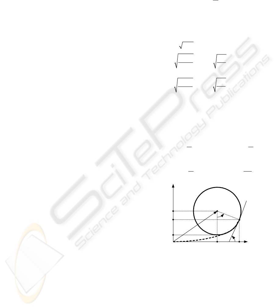
Figure 5: Transition from a straight line to a circumference
arc using a clothoid curve. m represents the distance
between the straight line and the circumference.
The smooth transition from a straight line to a
circumference is shown in Fig. 5, where the
x
−
axis
represents a straight line tangent to the clothoid
trajectory. The dashed line clothoid curve should
handle the smooth transition between the straight
line and the circumference arc with centre at
()
,
cc
x
y
,
SMOOTH TRAJECTORY PLANNING FOR FULLY AUTOMATED PASSENGERS VEHICLES - Spline and Clothoid
based Methods and its Simulation
93
radius and curvature
l
r
1
l
kr=
. Solving the equations,
one can find the clothoid parameters
σ
and :
l
2
1
2
ll
r
σ
θ
= and
2
ll
lr
θ
=
. (15)
Trajectory
Planning
Methods
θ
=
h (x, y)
θ
y
(t)
Processing
v
ri
Δ
t
i
=
f
( x
i
,
y
i
,
v
r i
)
Δ
t
i
x
i
y
i
x
(t)
v (t)
θ
(
t)
y
x
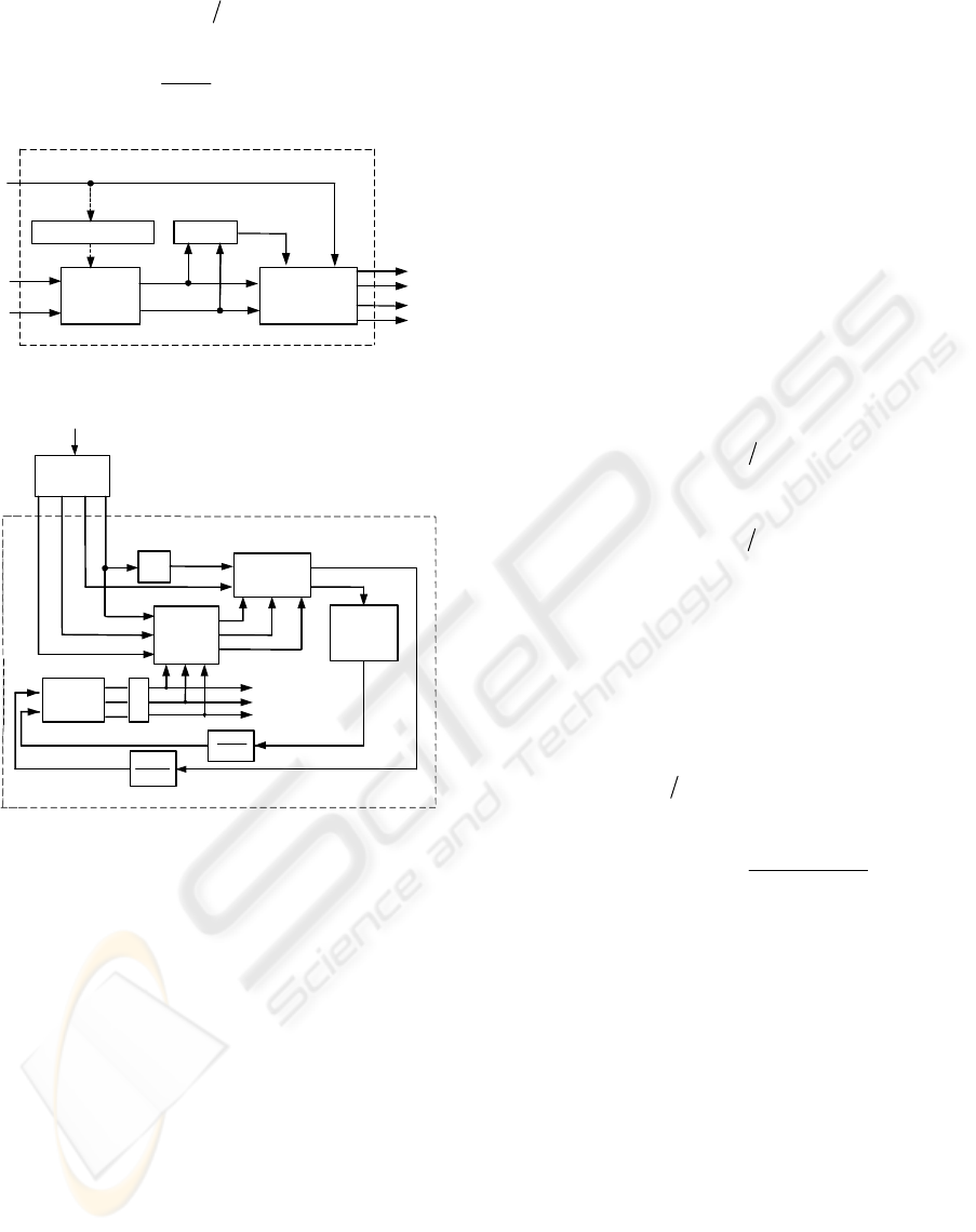
Trajectory Planning
Figure 6: Trajectory planning module.
Trajectory
Planning
Steering
Calculation
Controller
Kanayama
Error
Vehicle
Kinematic
Model
d / dt
V
r
V
V
ϕ
ϕ
ω
ω
r
x
c
x
c
y
c
y
c
y
e
x
e
θ
c
θ
c
θ
e
x
i
y
i
v
ri
1
1
+
v
s
τ
1
1
+
τ
s
∫
θ
r
x
r
y
r
θ
r
V
r
x
r
y
r
ϕ
Simulation Model
Figure 7: Simulation model block diagram: trajectory
planning and trajectory-tracking modules.
The trajectory planning using clothoids is not an
interpolation method. The trajectory results from the
concatenation of straight line segments, clothoid
curves, and circumference arcs. Thus, the trajectory
is obtained by means of a geometric construction,
and it is not possible to use the prescribed points in
the same way as in interpolation methods. A
previous processing is needed for assigning new
points, circumference arcs radius, and the distance
between the straight line segments and
circumference arcs.
5 SIMULATION MODEL
A simulation numerical model was developed using
the MATLAB/SIMULINK programming
environment (see Figs. 6 and 7). The first step
consisted on calculating the trajectories, from a set
of points
(
)
,, 1,2,,
iii
pxyi n
=
=…
, using cubic splines,
trigonometric splines and clothoids. These
calculations give the reference positions x and y. A
time vector is obtained from the desired trajectory
speed values which is used to define the time
depending reference variables
ri
v
(), (), ()
x
tyt t
θ
and
, as shown in Fig.6. A trajectory controller must
ensure that the vehicle follows the planned reference
trajectory. Errors are obtained comparing the
reference position with vehicle’s position, and a
Kanayama controller (Kanayama 1991) is used to
calculate velocity commands and
()vt
v
ω
. The angle
ϕ
is calculated in order to model the steering input of a
car-like vehicle. For a front wheels only steering,
0k
=
,
arctan( )
L
v
ϕ
ω
=
⋅
. (16)
while for both front and rear wheels steering, and for
equal front and rear angles, , results:
1k =
arcsin( 2 )
L
v
ϕ
ω
=
⋅
. (17)
For other values of it is more complicated to find
the value of angle
k
ϕ
. One possible way is to expand
the sine and cosine in Taylor series and solve the
resulting equation. The kinematics model (9) is
related to the velocity this velocity is in the
direction of the rear wheels, as shown in Fig. 3. On
the other hand, the target velocity is in the direction
of the vehicle axis. Hence,
T
v
cos( )
T
vv k
ϕ
=
(18)
and the kinematics model becomes
2
sin( )
cos sin
.cos
T
T
FF
T
F
x
k
yv
L
ϕϕ
θθ
ϕ
θ
⎡⎤
⎡
⎤
+
=
⎢⎥
⎢
⎥
⎢⎥
⎣
⎦
⎣⎦
(19)
Simple first order steering and speed vehicle’s
model were used in simulations, using time
constants
ϕ
τ
and
v
τ
between the reference and the
targets angle
ϕ
and velocity
v
(see Fig.7).
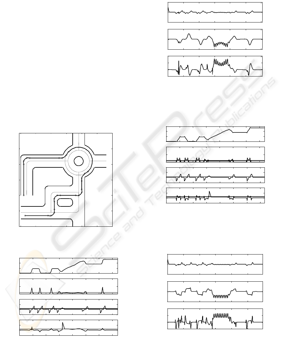
6 RESULTS
Three trajectory planning methods were applied to a
set of prescribed waypoints (points defined by stars
in Fig. 4). These point locations represent an urban
road way with very close corners and a roundabout.
As an example, a planned trajectory using
trigonometric splines is depicted in Fig. 8. Figs. 9 to
14 show results of the trajectory planning and
ICINCO 2006 - ROBOTICS AND AUTOMATION
94
vehicle's path-following for the three trajectories
obtained using the planning methods described in
Section 4.
Figures 9, 11 and 13 show the orientation angle,
curvature, and longitudinal and lateral accelerations
behaviour. The curvature is a non time-depending
parameter, which shows the smoothness of the
planned curve. The acceleration results allow an
evaluation of the trajectory comfort. However, the
accelerations also depend on linear speed variation.
So, using a different speed profile other results
would be obtained. Subsequently, the planned
trajectories were applied to the simulation model for
trajectory tracking, using a Kanayama controller.
The tracking errors obtained from the simulation are
shown in Figs. 10, 12 and 14. The angle,
longitudinal and lateral errors are shown for cubic
splines, trigonometric splines and clothoid curves
planned trajectories tracking. Table 2 summarises
results of the applied trajectory planning methods.
0 10 20 30 40 50 60
0
10
20
30
40
50
60
x (m)
y (m)
Figure 8: Generated trajectory using trigonometric splines.
0 20 40 60 80 100 120 140
0
100
200
300
Angle teta
(degree)
0 20 40 60 80 100 120 140
0
1
2
Curvature
(1/m)
0 20 40 60 80 100 120 140
-1
0
1
2
Longitudinal
acceleration
(m/s2)
0 20 40 60 80 100 120 140
-1
0
1
2
Length of course (m)
Lateral
acceleration
(m/s2)
r.m.s.
r.m.s.
r.m.s.
Figure 9: Orientation angle
θ
, curvature, longitudinal and
lateral acceleration behaviour along the course for the
given reference velocity vector, using cubic splines
trajectory planning.
0 20 40 60 80 100 120
-0.5
0
0.5
Longitudinal
error (m)
0 20 40 60 80 100 120
-0.5
0
0.5
Lateral
error (m)
0 20 40 60 80 100 120
-10
0
10
20
Tim e (s )
Angle
error (degree)
Figure 10: Angle, longitudinal and lateral tracking errors,
using a Kanayama controller and the vehicle kinematics
model to follow cubic splines planned trajectory.
0 20 40 60 80 100 120 140
0
100
200
300
Angle teta
(degree)
0 20 40 60 80 100 120 140
0
1
2
Curvature
(1/m)
0 20 40 60 80 100 120 140
-1
0
1
2
Longitudinal
acceleration
(m/s2)
0 20 40 60 80 100 120 140
-1
0
1
2
Length of course (m)
Lateral
acceleration
(m/s2)
r.m.s.
r.m.s.
r.m.s.
Figure 11: Orientation angle
θ
, curvature, longitudinal
and lateral acceleration behaviour along the course for the
given reference velocity vector, using trigonometric
splines trajectory planning.
0 20 40 60 80 100
-0.5
0
0.5
Longitudinal
error (m)
0 20 40 60 80 100
-0.5
0
0.5
Lateral
error (m)
0 20 40 60 80 100
-10
0
10
20
Time (s )
Angle
error (degree)
Figure 12: Angle, longitudinal and lateral tracking errors,
using a Kanayama controller and the vehicle kinematics
model to follow cubic trigonometric planned trajectory.
SMOOTH TRAJECTORY PLANNING FOR FULLY AUTOMATED PASSENGERS VEHICLES - Spline and Clothoid
based Methods and its Simulation
95
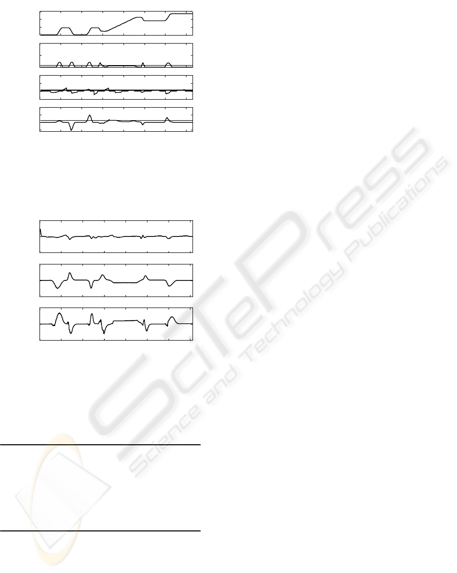
0 20 40 60 80 100 120 140
0
100
200
300
Angle teta
(degree)
0 20 40 60 80 100 120 140
0
1
2
Curvature
(1/m)
0 20 40 60 80 100 120 140
-1
0
1
2
Longitudinal
acceleration
(m/s2)
0 20 40 60 80 100 120 140
-1
0
1
2
Length of course (m)
Lateral
acceleration
(m/s2)
r.m.s.
r.m.s.
Figure 13: Orientation angle
θ
, curvature, longitudinal
and lateral acceleration behaviour along the course for the
given reference speed profile, using clothoid curves
trajectory planning.
0 20 40 60 80 100 120 140
-0.5
0
0.5
Longitudinal
error (m)
0 20 40 60 80 100 120 140
-0.5
0
0.5
Lateral
error (m)
0 20 40 60 80 100 120 140
-10
0
10
Time (s )
Angle
error (degree)
Figure 14: Angle, longitudinal and lateral tracking errors,
using a Kanayama controller and the vehicle kinematics
model to follow clothoid curves planned trajectory.
Table 2: Planning Methods Results.
Quantity Cub. Trig. Clothoid
Max. Curvature (1/m) 0.87 0.56 0.41
r.m.s. Curvature (1/m) 0.21 0.20 0.16
Max. Long. Accel. (m/s
2
) 0.69 0.69 0.42
r.m.s. Long. Accel. (m/s
2
) 0.21 0.21 0.15
Max. Lateral Accel. (m/s
2
) 1.50 1.32 0.95
r.m.s. Lateral Accel. (m/s
2
) 0.24 0.25 0.25
Overall Acceleration (m/s
2
) 0.43 0.46 0.40
7 CONCLUSIONS
In this paper, three trajectories planning methods
using cubic splines, trigonometric splines and
clothoid curves, were analysed. The integration of a
speed profile planner was proposed, with the goal of
calculating the time-intervals sequence that lead to
low level of accelerations and jerk. Further research
is being carried out in this direction (Solea 2006).
The generated trajectories were applied to a numeric
model for trajectory-tracking, using a Kanayama
controller. The first conclusion is related to the use
of methods easiness. In spite of the relatively good
results, the use of clothoid curves is complex and
without flexibility in case of trajectory change. On
the other hand, all methods showed to be adequate
from the point of view of passengers' comfort and
tracking.
ACNOWLEDGEMENTS
This wok was supported in part by ISR-UC and FCT
(Fundação para a Ciência e Tecnologia), under
contract NCT04: POSC/EEA/SRI/58016/2004
.
REFERENCES
Bishop, R., 2005. Intelligent Vehicle Technology and
Trends, Artech House.
Cybercars 2001. Cybernetic technologies for the car in the
city. [online], www.cybercars.org.
Gerald, C. and P. Wheatley, 1984. Applied Numerical
Analysis, Menlo Park, California, Addison-Wesley.
Kanayama, Y., Y. Kimura, F. Miyazaky and T. Noguchy,
1991. A stable tracking control method for a non-
holonomic mobile robot. IEEE/RSJ Int. Conference on
Intelligent Robots and Systems (IROS 1991).
Leao, D., T. Pereira, P. Lima and L. Custódio, 2002.
Trajectory planning using continuous curvature paths,
Journal DETUA, Vol.3, nº6, (in Portuguese).
Nagy, M. and T. Vendel , 2000. Generating curves and
swept surfaces by blended circles. Computer Aided
Geometric Design, Vol. 17, 197-206.
Parent, M., G. Gallais, A. Alessandrini, T.Chanard, 2003.
CyberCars: review of first projects. Int. Conference on
People Movers APM 03. Singapore.
Piazzi, A., and A. Visioli, 2000. Global minimum-jerk
trajectory of robot manipulators. IEEE Transactions
on Industrial Electronics. Vol. 47, nº1, 140-149.
Solea, R., and U. Nunes, 2006. Trajectory planning with
embedded velocity planner for fully-automated
passenger vehicles. IEEE 9
th
Intelligent
Transportation Systems Conference. Toronto, Canada.
Rodrigues, R., F. Leite, and S. Rosa, 2003. On the
generation of a trigonometric interpolating curve in
ℜ
3
, 11th Int. Conference on Advanced Robotics,
Coimbra, Portugal.
Sekhavat, S. and J. Hermosillo 2000. The Cycab robot: a
differentially flat system. IEEE/RSJ Int. Conf. on
Intelligent Robots and System (IROS 2000).
ICINCO 2006 - ROBOTICS AND AUTOMATION
96
