ON JUST IN TIME CONTROL OF SWITCHING MAX-PLUS

LINEAR SYSTEMS

Michel Alsaba, S

ebastien Lahaye and Jean-Louis Boimond

LISA

62 avenue Notre Dame du Lac - Angers, France

Keywords:

Discrete event systems, (max, +) algebra, switching max-plus linear systems, just in time control.

Abstract:

Discrete event systems involving synchronization and delay phenomena can be described by a linear state rep-

resentation over (max, +) algebra. Some discrete event systems involving choice phenomena could be trans-

formed, under some conditions, into switching max-plus linear systems modeled as automata. The switching

between states of these automata is governed by a switching variable. This paper deals with the just in time

control of these switching max-plus linear systems. The control problem we propose is optimal under just in

time criterion when the switching variable is given on the study horizon.

1 INTRODUCTION

The class of Discrete Event Systems (DES) essen-

tially consists of man-made systems that contain a ﬁ-

nite number of ressources (such as machines, commu-

nications channels, or processors) shared by several

users (such as product types, information packets, or

jobs) all of which contributing to the achievement of

some common goal as the assembly of products, the

end to end transmission of a set of information pack-

ets, or a parallel computation, (Baccelli et al., 1992).

In general, models of DES are nonlinear in conven-

tional algebra. However, there exists a class of DES

which have been shown to be linear in a particular al-

gebraic structure, namely max-plus algebra (Baccelli

et al., 1992). The so-called max-plus linear systems

involve only synchronization and delay phenomena

(but no conﬂict) which are basically modeled by max-

imization and addition operations. Regarding Timed

Petri Nets (TPN) which enable to model (and partly

analyze) a wide variety of DES, max-plus linear sys-

tems mainly ﬁt to the subclass of Timed Event Graphs

(TEG).

Several studies have attempted to widen the class

of DES likely to be analyzed thanks to max-plus al-

gebraic tools. Among those works, we focus in this

paper on the so-called switching max-plus linear sys-

tems which have been introduced in (van den Boom

and de Schutter, 2004). They can be seen as an au-

tomaton switching between several max-plus linear

state representations. They are an adequate tool to

model DES in which several modes of operation take

effect. Beside max-plus linear models, switching al-

low to take into account additional phenomena such

as breaks of synchronization and changes in events

occurrences order. In (van den Boom and de Schutter,

2004), authors have proposed a model predictive con-

trol for such systems to optimize their behavior. In

this paper, we tackle another control problem, namely

the output tracking problem with respect to just in

time criterion. This control have been extensively

studied for max-plus linear systems notably in (Cohen

et al., 1989), (Menguy et al., 2000). Under particular

assumptions, we show that switching max-plus lin-

ear systems admit representations and a just-in-time

control solution inspired by those of max-plus linear

time-varying systems (Lahaye et al., 1999). The con-

tribution lies in the possibility to take into account

changes in the system structure while only parame-

ters may vary in the time-varying case.

This paper is organized as follows. Some results

used in the sequel are recalled in the second section.

A general presentation about switching max-plus lin-

ear systems is given in the third section. We expose

the JIT control problem of such systems in the fourth

section. We give two applications in the ﬁfth section.

Alsaba M., Lahaye S. and Boimond J. (2006).

ON JUST IN TIME CONTROL OF SWITCHING MAX-PLUS LINEAR SYSTEMS.

In Proceedings of the Third International Conference on Informatics in Control, Automation and Robotics, pages 79-84

DOI: 10.5220/0001204200790084

 SciTePress

2 PRELIMINARIES

2.1 Algebraic Tools

2.1.1 Dioid

See (Cohen et al., 1989), (Baccelli et al., 1992, §4) for

an exhaustive presentation of dioid theory.

A dioid (D, ⊕, ⊗) is an idempotent

semiring, neu-

tral elements of ⊕ and ⊗ are denoted ε and e respec-

tively. The symbol ⊗ is often omitted.

A dioid D is complete if it is closed for inﬁnite

sums and if the product distributes over ﬁnite and in-

ﬁnite sums. The upper bound of a complete dioid,

denoted ⊤ (for Top), is the sum of all dioid elements

and it is absorbing for the addition.

An order relation, noted , can be associated with

a dioid D by the following equivalence: ∀ a, b ∈

D, a  b ⇔ a = a ⊕ b. This order relation con-

fers upon complete dioid a structure of complete lat-

tice. So, we can introduce an operator Inf, denoted

∧, verifying:

∀ a, b ∈ D, a  b ⇔ b = a ∧ b.

Example 1 The set Z ∪ {−∞, +∞}, endowed with

the max operator as additive law and the classical

sum as product, is a complete dioid, usually denoted

max

, with ε = −∞, e = 0 and ⊤ = +∞.

If D is a dioid, the set D

n×n

of n × n matri-

ces with coefﬁcients in D is also a dioid. Sum

and product are deﬁned in the following way:

(A ⊕ B)

= A

⊕ B

, (A ⊗ B)

k=1

⊗ B

Theorem 1 Over a complete dioid D, the implicit

equation x = ax ⊕ b admits a

∗

b as least solution

where a

∗

i∈N

with a

= e.

2.1.2 Residuation Theory

A complete presentation of this theory is given in

(Blyth and Janowitz, 1972), see (Baccelli et al., 1992,

§4.4) for a specialization to dioid.

Residuation theory provides, under some assump-

tions, the greatest solution to inequality f(x)  b,

where f is an isotone mapping

deﬁned over ordered

sets.

An isotone mapping f : D → F, where (D, 

)

and (F, 

) are ordered sets, is a residuated mapping

if for all b ∈ F the upper bound of the subset {x ∈

D|f(x) 

b} exists and belongs to this subset.

Theorem 2 Let f : D → F be an isotone mapping

from the complete dioid (D, 

) into the complete

dioid (F, 

). The following statements are equiva-

lent:

∀a ∈ D, a ⊕ a = a.

f is an isotone mapping if a  b ⇒ f (a)  f(b).

(i) f is residuated.

(ii) There exists a unique isotone mapping f

♯

: F →

D, called residual, such that f ◦ f

♯



and

♯

◦f 

where id

and id

are identity map-

pings in F and D respectively.

Example 2 Mappings L

: x 7→ a ⊗ x and

: x 7→ x ⊗ a deﬁned over a complete dioid D are

both residuated. Their residuals are usually denoted

by L

♯

(x) = a

◦

\x and R

♯

(x) = x

◦

/a respectively.

These ’quotients’ satisfy the following formulae:

a ⊗ (a

◦

\x)  x, (x

◦

/a) ⊗ a  x, (i)

◦

\(x ∧ y) = (a

◦

\x) ∧ (a

◦

\y), (ii)

(x ∧ y)

◦

/a = (x

◦

/a) ∧ (y

◦

/a), (iii)

(a ⊗ b)

◦

\x = b

◦

\(a

◦

\x), x

◦

/(a ⊗ b) = (x

◦

/b)

◦

/a. (iv)

3 LINEAR SYSTEMS

3.1 Max-plus Linear Systems

It has been shown that DES involving synchronization

and delay phenomena (but no choice phenomenon)

can be described by a linear state representation over

dioid

max

(see (Baccelli et al., 1992) for a detailed

presentation):



x(k) = A(k )x(k − 1) ⊕ B(k)u(k),

y(k) = C(k)x(k).

(1)

Such systems are usually referred to as (max, +)

linear systems. The index k is called the event

counter. Entries of state vector x(k) are daters func-

tions expressing the time instants at which the internal

events occur for the k-th time. Similarly, vectors u(k)

and y(k ) contain daters associated respectively with

input and output events.

3.2 Switching Max-plus Linear

Systems

We now consider so-called switching max-plus linear

systems introduced and studied in (van den Boom and

de Schutter, 2004). This class of systems corresponds

to DES that can switch between different modes of

operation. In each mode l = 1, ..., q, the system is

described by a (max, +) linear state space model:

x(k) = A

(l)

(k )x(k − 1) ⊕ B

(l)

(k )u(k),

y(k) = C

(l)

(k )x(k).

(2)

in which the matrices A

(l)

, B

(l)

and C

(l)

are the sys-

tem matrices for the l-th mode. In general the switch-

ing allows to model a change in the structure of the

system, such as breaking a synchronization or chang-

ing the events occurrences order (several examples are

proposed in (van den Boom and de Schutter, 2004)).

ICINCO 2006 - SIGNAL PROCESSING, SYSTEMS MODELING AND CONTROL

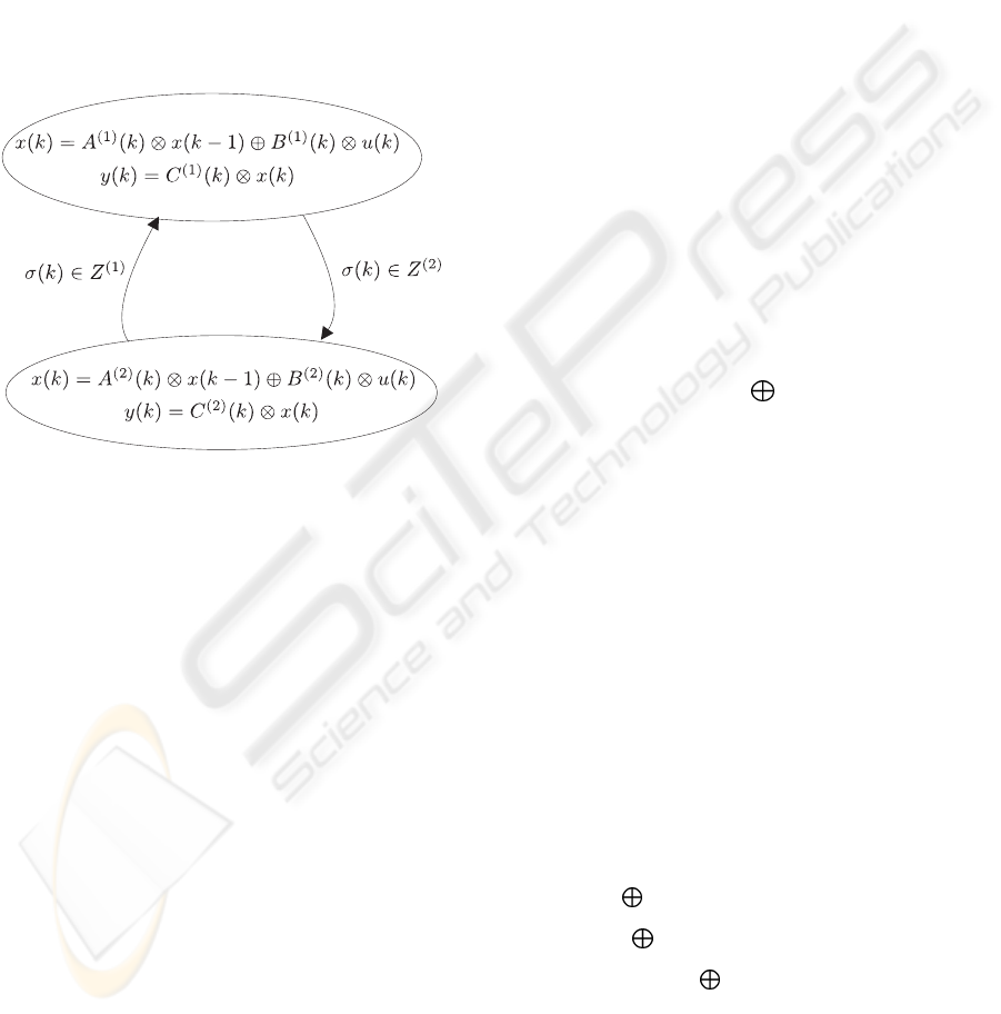
The moments of switching are determined by a

switching mechanism. A switching variable σ(k)

is deﬁned, which may depend on the previous state

x(k − 1), the previous mode l(k − 1), the input vari-

able u(k) and/or an external decision variable v(k):

σ(k) = Φ(x(k − 1), l(k − 1), u(k), v(k)) ∈ R

. (3)

Set R

is partitioned in q subsets Z

(i)

, i = 1 . . . q.

The mode l(k) is now obtained by determining in

which subset σ(k) is for event k. So if σ(k) ∈ Z

(i)

then l(k ) = i. We represent on ﬁgure 1 a simple

switching max-plus linear system with two modes.

Figure 1: A simple switching max-plus linear system.

4 REPRESENTATIONS AND JUST

IN TIME CONTROL OF

SWITCHING MAX-PLUS

LINEAR SYSTEMS

In this section, we ﬁrst focus on representations of

switching max-plus linear systems. Assuming that

the switching variable is known on the study hori-

zon, we explicit the solution of state equation (2) and

identify its impulse response. The obtained represen-

tations are reminiscent of those of (max, +) linear

time-varying systems (Lahaye et al., 1999), except

that structures of implied matrices may vary along

evolution in the switching case, while only parame-

ters may vary in the time-varying case.

From these representations, we can next tackle a

control problem for switching max-plus linear sys-

tems, namely the output tracking problem with re-

spect to just in time criterion.

4.1 Representations

In the following, we assume that switching variable

σ(k) is known on the study horizon. Referring to

equation (3), this may happen in particular if:

1. σ(k) = Φ(v(k)), in which the external decision

variable v(k) is supposed to be given on the study

horizon.

2. σ(k) = Φ(l(k − 1)), where function l(k), stating

the mode at step k according to the previous one, is

supposed to be given on the study horizon.

So the ﬁrst equation of (2) can be written for k ≥

x(k) = Φ(k, k

)x(k

) ⊕

j=k

Φ(k, j)B

(l)

(j)u(j)

where Φ(k, i) is the transition matrix given by:

Φ(k, i) =







not deﬁned if i > k,

Id if i = k,

(l)

(k )A

(l)

(k − 1)...A

(l)

(i + 1) otherwise.

Then, we deduce the output:

y(k) = C

(l)

(k)Φ(k, k

)x(k

) ⊕

j=k

(l)

(k)Φ(k, j)B

(l)

(j)u(j)

(4)

Remark 1 The state-transition matrix satisﬁes the

composition property

Φ(k, i) = Φ(k, j) ⊗ Φ(j, i), where k ≥ j ≥ i,

and in particular for k ≥ i + 1

Φ(k, i) = A

(l)

(k)Φ(k−1, i) = Φ(k, i+1)A

(l)

(i+1).

Proposition 1 The least solution of equations (2) is

given by ∀k ∈ Z, ¯y(k) =

j≤k

h(k, j)u(j) with

h(k, j) = C

(l)

(k)Φ(k , j)B

(l)

(j), for j ≤ k.

h is called the impulse response of the system.

Proof By tending k

towards −∞ in equation (4),

it is clear that any solution is greater than ¯y.

Setting ¯y(k ) = C

(l)

(k)¯x(k) with

¯x(k) =

j≤k

Φ(k, j)B

(l)

(j)u(j),

We show that ¯x satisﬁes the ﬁrst equation of (2):

¯x(k) =

j≤k

Φ(k, j)B

(l)

(j)u(j),

j≤k−1

Φ(k, j)B

(l)

(j)u(j) ⊕ B

(l)

(k )u(k),

= A

(l)

(k )[

j≤k−1

Φ(k − 1, j)B

(l)

(j)u(j)]

⊕B

(l)

(k )u(k), (thanks to remark 1)

= A

(l)

(k )¯x(k − 1) ⊕ B

(l)

(k )u(k). 

ON JUST IN TIME CONTROL OF SWITCHING MAX-PLUS LINEAR SYSTEMS

4.2 Just In Time Control of

Switching Max-plus Linear

Systems

4.2.1 Description

Strong analogies appear between the classical linear

system theory and the (max, +) linear system the-

ory. In particular, the concept of control is now well

deﬁned for these systems. A greatest control, based

on residuation theory (Blyth and Janowitz, 1972), has

been proposed in (Cohen et al., 1989), (Menguy et al.,

2000). For a given reference input (i.e., desired dates

of occurrence for output events) Z = {z(k)}

k=0,..,k

the control yields the latest dates of occurrence for

input events U = {u(k)}

k=0,..,k

in order that the

output events Y = {y(k)}

k=0,..,k

occur before the

reference input. Such a greatest control is called

Just In Time (JIT) control. In a production context,

it amounts to satisfying the customer demand while

minimizing the stocks. Using representations pro-

posed at section 4.1, we propose a JIT control for

switching Max-plus linear systems.

4.2.2 Control Problem for Switching Max-plus

Linear Systems

Proposition 2 From proposition 1, the output y of a

switching max-plus linear system can be written as

y = H(u) where [H(u)](k) =

j≤k

h(k, j)u(j).

Then the JIT optimal control, denoted u

opt

(k), is

given by:

opt

(k) = [H

♯

(z)](k) =

j≥k

h(j, k)

◦

\z(j).

Proof We denote ω the signal deﬁned by:

∀k ∈ Z, ω(k) =

j≥k

h(j, k)

◦

\z(j).

1. Let x satisfying H(x)  Z or equivalently,

∀k ∈ Z,

i∈Z

h(k, i)x(i) =

i≤k

h(k, i)x(i)  z(k)

∀k, i ∈ Z, i ≤ k; h(k, i)x(i)  z(k)

∀k, i ∈ Z, i ≤ k; x(i)  h(k, i)

◦

\z(k)

∀i ∈ Z, x(i) 

k≥i

h(k, i)

◦

\z(k) = ω(i)

2. Using (i),∀k ∈ Z,

i∈Z

h(k, i)ω(i) =

i∈Z

h(k, i)[

j≥i

h(j, i)

◦

\z(j)] 

i∈Z

h(k, i)[h(k, i)

◦

\z(k)] 

i∈Z

z(k) = z(k) which

shows that ω is solution of H(x)  Z. 

In the following, we show that u

opt

is solution

of a system of recurrent equations which proceed

backwards in event index. These equations offer a

strong analogy with the adjoint-state equations of

optimal control theory. Firstly let us remark using

(iv) that:

opt

(k ) =

j≥k

h(j, k)

◦

\z(j)

j≥k

(l)

(j)Φ(j, k)B

(l)

(k ))

◦

\z(j)

j≥k

(l)

(k )

◦

\[(C

(l)

(j)Φ(j, k))

◦

\z(j)]

= B

(l)

(k )

◦

when setting

ξ(k) =

j≥k

(l)

(j)Φ(j, k))

◦

\z(j).

Proposition 3 The greatest solution of equation:

ξ(k) = A

(l)

(k + 1)

◦

\ξ(k + 1) ∧ C

(l)

(k )

◦

\z(k) (5)

is given by:

ξ(k) =

j≥k

(l)

(j)Φ(j, k))

◦

\z(j).

Proof

1. Let us ﬁrst show that

ξ is solution of equation (5).

∀k ∈ Z,

(l)

(k + 1)

◦

ξ(k + 1) ∧ C

(l)

(k)

◦

\z(k)

= A

(l)

(k + 1)

◦

i≥k+1

(l)

(i)Φ(i, k + 1))

◦

\z(i)] ∧

(l)

(k)

◦

\z(k)

i≥k+1

(l)

(i)Φ(i, k + 1)A

(l)

(k + 1))

◦

\z(i) ∧

(l)

(k)

◦

\z(k) (thanks to (ii) and (iv))

i≥k+1

(l)

(i)Φ(i, k))

◦

\z(i) ∧

(l)

(k)Φ(k , k ))

◦

\z(k) (see remark 1)

i≥k

(l)

(i)Φ(i, k))

◦

\z(i) (thanks to (ii))

ξ(k)

2. Let {ξ(k)}

k∈Z

a solution of equation (5), we have

∀k ∈ Z

ξ(k) = Φ(k + k

, k)

◦

\ξ(k + k

) ∧

k+k

−1

j=k

(l)

(j)Φ(j, k))

◦

\z(j), k

≥ 1.

With k

→ +∞, it is clear that ∀k, ξ(k) 

ξ(k). 

So ﬁnally, {u

opt

(k)}

k∈Z

can be computed us-

ing the following backward iterative procedure:



ξ(k) = A

(l)

(k + 1)

◦

\ξ(k + 1) ∧ C

(l)

(k )

◦

\z(k),

opt

(k ) = B

(l)

(k )

◦

\ξ(k).

5 APPLICATION

5.1 Example 1

This is a generic example because in much industrial

applications (specially in ﬂexible manufacturing sys-

ICINCO 2006 - SIGNAL PROCESSING, SYSTEMS MODELING AND CONTROL

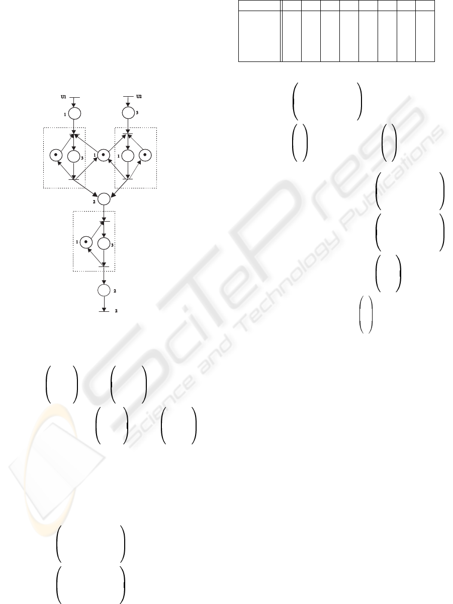
tems) we ﬁnd shared resources (as a welding or paint-

ing robot shared between production lines). Output

parts of this stage are processed by the machine M3.

Using Petri nets to model shared resources leads to a

structure of choice represented by a place P (see ﬁg-

ure 2) with an input fork of arcs and another one out-

going. The three machines used M1, M 2, M3 have

one server each, which means that each one treats one

product at once. Processing times on machines M

and M

are respectively 3, 1 and 3 units of time.

Figure 2: Petri net model for example 1.

If l(k) = 1 then u(k) = U

(k),

x(k) =

(k )

X1(k )

X3(k )

X5(k )

X6(k )

else

u(k) = U

(k),

x(k) =

(k )

X2(k )

X4(k )

X5(k )

X6(k )

Considering the ﬁrst case which means l(k) = 1

we will give how we can extract the state space

equations:

(k) = 1x

(k − 1) ⊕ 1u(k),

(k) = 3x

(k),

(k) = 2x

(k) ⊕ 1x

(k − 1),

(k) = 3x

(k),

Y (k) = x

(k),

(1)

(k ) =

ε ε ε ε

3 ε ε ε

ε 2 ε ε

ε ε 3 ε

(2)

(k ) =

ε 1 ε ε

ε ε ε ε

ε ε ε 1

ε ε ε ε

Table 1: Numerical data and optimal control for system rep-

resented on ﬁgure 2.

k 0 1 2 3 4 5 6 7

z(k) 21 22 24 25 29 33 35 39

l(k) 2 1 1 1 2 1 2 2

opt

(k)

4 8 12 20

opt

(k)

0 16 24 28

y(k) 11 15 19 23 27 31 35 39

(3)

(k ) =

ε ε ε ε

1 ε ε ε

ε 2 ε ε

ε ε 3 ε

(1)

(k ) =

(2)

(k ) =

Now using theorem 1, we get:

(1)

(k ) = (α

(1)

∗

) ⊗ α

(2)

ε 1 ε ε

ε 4 ε ε

ε 6 ε 1

ε 9 ε 4

(2)

(k ) = (α

(3)

∗

) ⊗ α

(2)

ε 1 ε ε

ε 2 ε ε

ε 4 ε 1

ε 7 ε 4

(1)

(k ) = (α

(1)

∗

) ⊗ β

(1)

in the same way we get: B

(2)

(k) =

Considering that the switching variable σ(k) is

known on the horizon of study, and consequently l(k)

will be known too, so we can apply the proposed

method for a just in time control. Table 1 shows a

numerical experimentation: z(k) corresponds to the

desired delivery date for the k-th ﬁnished piece, l(k)

gives the machine number which treats the k-th part,

opt

(·) and u

opt

(·) are the computed optimal in-

puts, and y(·) is the output response to u

opt

(·) and

opt

(·). We verify that for all k we have y(k) 

z(k).

5.2 Example 2

We consider a manufacturing system consisting of

three machines. It is supposed to produce one kind

of piece by assembling two kinds of raw parts de-

noted P

and P

. Two modes can be chosen along

production. In a ﬁrst mode, parts P

(resp. P

)

are preprocessed on machine M

(resp. M

) and ﬁ-

nally assembled and processed on machine M

. In

the second mode, parts P

and P

are assembled and

preprocessed on machine M

, and then processed

successively by machines M

and M

. Routings

ON JUST IN TIME CONTROL OF SWITCHING MAX-PLUS LINEAR SYSTEMS

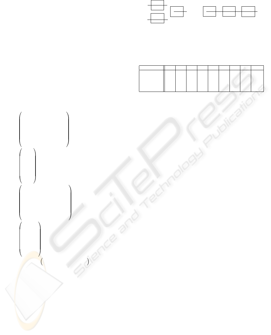
of parts are depicted on ﬁgure 3. When a switch

between modes occurs, we assume that semi-ﬁnite

pieces preprocessed by machines 1 and 2 (stocked in

their downstream buffers) can be processed indiffer-

ently by downstream machines in the new mode. Fur-

thermore, we assume that there are no set-up-times

on machines when they switch from one mode to an-

other. Processing times on machines M

, M

and M

are respectively 3, 4 and 5 units of time.

Functioning of the system can be represented by

a max-plus linear state equation (2) speciﬁc to each

mode. In both modes, we associate two input daters

denoting dates at which raw parts P

and P

are

released in production. Six state daters are used to

respectively represent input and output dates of parts

on machines M

, M

and M

. Finally, one output

dater denotes delivering dates of ﬁnished parts. We

get the following representations:

(1)

(k) =

ε 0 ε ε ε ε

ε 3 ε ε ε ε

ε ε ε 0 ε ε

ε ε ε 4 ε ε

ε 3 ε 4 ε 0

ε 8 ε 9 ε 5

(1)

(k) =

0 ε

3 ε

ε 0

ε 4

3 4

8 9

(2)

(k) =

ε 0 ε ε ε ε

ε 3 ε ε ε ε

ε 3 ε 0 ε ε

ε 7 ε 4 ε ε

ε 7 ε 4 ε 0

ε 12 ε 9 ε 5

(2)

(k) =

0 0

3 3

7 7

12 12

(1)

(k) = C

(2)

(k) =

ε ε ε ε ε 0

Considering that the switching variable σ(k) is

known on the horizon of study, and consequently l(k)

will be known too, so we can apply the proposed

method for a just in time control. Table 2 shows a

numerical experimentation: z(k) corresponds to the

desired delivery date for the k-th ﬁnished piece, l(k)

gives the mode of production chosen for the k-th part,

opt

(·) and u

opt

(·) are the computed optimal in-

puts, and y(·) is the output response to u

opt

(·) and

opt

(·). We verify that ∀k we have y(k)  z(k).





Mode 1

Mode 2

Figure 3: Routings of parts along machines according to

modes of production.

Table 2: Numerical data and optimal control for example 2.

k 0 1 2 3 4 5 6 7 8

z(k) 15 20 35 45 60 75 80 95 100

l(k) 1 1 2 2 2 1 2 1 2

opt

(k) 7 12 27 37 52 67 72 85 88

opt

(k)

6 11 26 36 51 66 71 86 88

y(k) 15 20 35 45 60 75 80 95 100

6 CONCLUSION

In this paper we have considered the just in time con-

trol problem of switching max-plus linear systems.

The proposed control is optimal under just in time

criterion in the case where the switching variable is

given on the study horizon. In futur work, we will

consider a different switching variable more general

which is not necessarily given from the beginning.

REFERENCES

Baccelli, F., Cohen, G., Olsder, G.-J., and Quadrat, J.-P.

(1992). Synchronization and Linearity: An Algebra

for Discrete Event Systems. Wiley and Sons.

Blyth, T. and Janowitz, M. (1972). Residuation Theory.

Pergamon press.

Cohen, G., Moller, P., Quadrat, J.-P., and Viot, M. (1989).

Algebraic Tools for the Performance Evaluation of

Discrete Event Systems. IEEE Proceedings: Special

issue on Discrete Event Systems, 77(1):39–58.

Lahaye, S., Boimond, J.-L., and Hardouin, L. (1999). Op-

timal Control of (Min,+) Linear Time-Varying Sys-

tems, Petri Nets and Performance Models. Proceed-

ings of PNPM’99, pages 170–178, Zaragoza, Spain.

Menguy, E., Boimond, J.-L., Hardouin, L., and Ferrier,

J.-L. (2000). Just-In-Time Control of Timed Event

Graphic Update of Reference Input, Presence of Un-

controllable Input. IEEE Trans. on Automatic Control,

45(11):2155–2158.

van den Boom, T. and de Schutter, B. (2004). Mod-

elling and Control of Discrete Event Systems Using

Switching Max-Plus-Linear Systems. In Proceedings

of WODES’04, pages 115–120, Reims, France.

ICINCO 2006 - SIGNAL PROCESSING, SYSTEMS MODELING AND CONTROL