
BAYESIAN ESTIMATION OF DISTRIBUTED PHENOMENA
USING DISCRETIZED REPRESENTATIONS OF
PARTIAL DIFFERENTIAL EQUATIONS
Felix Sawo, Kathrin Roberts and Uwe D. Hanebeck
Intelligent Sensor-Actuator-Systems Laboratory
Institute of Computer Science and Engineering
Universit
¨
at Karlsruhe (TH)
Karlsruhe, Germany
Keywords:
Stochastic systems, Baysian estimation, model-based reconstruction, distributed phenomenon, environmental
monitoring, sensor-actuator-network.
Abstract:
This paper addresses a systematic method for the reconstruction and the prediction of a distributed phenom-
enon characterized by partial differential equations, which is monitored by a sensor network. In the first step,
the infinite-dimensional partial differential equation, i.e. distributed-parameter system, is spatially and tempo-
rally decomposed leading to a finite-dimensional state space form. In the next step, the state of the resulting
lumped-parameter system, which provides an approximation of the solution of the underlying partial differen-
tial equations, is dynamically estimated under consideration of uncertainties both occurring in the system and
arising from noisy measurements. By using the estimation results, several additional tasks can be achieved
by the sensor network, e.g. optimal sensor placement, optimal scheduling, and model improvement. The
performance of the proposed model-based reconstruction method is demonstrated by means of simulations.
1 INTRODUCTION
Recent developments in wireless sensor network tech-
nology and miniaturization of sensor nodes make it
possible to exploit centralized (Kumar et al., 2002)
and decentralized (Rao et al., 1993) sensor networks
for monitoring the natural environment (Thuraising-
ham, 2004; Culler and Mulder, 2004). Such sensor
networks can be used for example in industrial, med-
ical, urban, and many other environments. Further-
more, applying sensor networks can provide new data
for environmental science, such as climate models, as
well as growth and reproduction of coral reef indi-
cated by physical environmental factors, e.g. temper-
ature, water movement, salt concentration, and pollu-
tant concentration. Further examples are reconstruc-
tion of fluid-flow in a thermal reactor (Faulds and
King, 2000), and reconstruction of the surface mo-
tion of a beating heart in minimally invasive surgery
(Ortmaier et al., 2005).
In practical implementations the sensor nodes are
normally densely deployed either inside the phenom-
enon or very close to it. In order to get meaningful in-
formation not only at the sensor nodes itself but also
between these nodes, the reconstruction of the distrib-
uted phenomenon is of major significance.
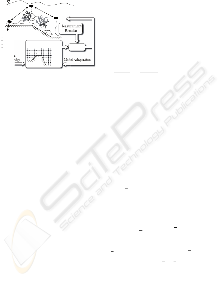
For the prediction of the state of such phenomenon
we present a new method for systematic data process-
ing. Basically, data from the sensor network in form
of measurement results as well as data from a physical
model are used to derive the best possible estimate for
the state of a distributed phenomenon; even at non-
measurement points. The estimation results on the
other hand can be used for finding the optimal place-
ment and measurement time sequences for the sensor
nodes, or for improving the parameter values of the
used physical model, see Fig. 1.
However, for a model-based approach it is neces-
sary to solve the partial differential equations char-
acterizing the distributed phenomena. Such equa-
tions can be solved for example by the finite-element
method or the finite-difference method (Baker, 1983).
The unstructured nature of those methods permits a
good geometrical description of complex geometries.
Additionally, it is possible to solve even nonlinear
partial differential equations. However, many para-
meters describing uniquely the state of the distrib-
uted phenomenon are necessary to achieve appropri-
ate convergence.
On the other hand, there are modal analysis meth-
ods using a set of global expansion functions. These
methods just need a few parameters for characterizing
16
Sawo F., Roberts K. and D. Hanebeck U. (2006).
BAYESIAN ESTIMATION OF DISTRIBUTED PHENOMENA USING DISCRETIZED REPRESENTATIONS OF PARTIAL DIFFERENTIAL EQUATIONS.
In Proceedings of the Third International Conference on Informatics in Control, Automation and Robotics, pages 16-23
DOI: 10.5220/0001203800160023
Copyright
c
SciTePress
Measurement
Results
Model Adaptation
A Priori
Knowledge
Stochastic Model
Fusion
Sensor node:
temperature
salt concen
tration
velocity
pressure
Sensor Scheduling and
Sensor Placement
Figure 1: Visionary scenario for the reconstruction and the
observation of a distributed phenomenon by means of a sen-
sor network; observation of a coral reef.
a smooth solution of the partial differential equation
(Roberts and Hanebeck, 2005). The drawback, how-
ever, is that the modal analysis works only for lin-
ear partial differential equations and global expansion
functions can be found only for problems with simple
boundary conditions.
Combining these two general approaches, leads to
the so-called finite-spectral method (Karniadakis and
Sherwin, 2005; Fournier et al., 2004; Levin et al.,
2000). Basically, this method approximates the so-
lution within each element with a set of orthogonal
polynomials, such as Legendre, or Chebyshev. Thus,
it combines the geometrical flexibility of conventional
finite-element methods with the exponential conver-
gence rate associated with the modal analysis.
The novelty of this paper is the model-based ob-
servation of distributed phenomena by a sensor net-
work under consideration of uncertainties both occur-
ing in the physical model, i.e., system model, and
arising from noisy measurements. Here, we extend
and generalize our previous research work (Roberts
and Hanebeck, 2005) in such a way that both the sys-
tem model and the measurement model are derived by
the finite-spectral method. Using this method, it turns
out that nonlinear phenomena with complex bound-
ary conditions can be reconstructed and predicted in a
systematic manner.
The remainder of this paper is organized as follows.
In Section II, a rigorous formulation of the problem
of the reconstruction of distributed phenomena char-
acterized by partial differential equations is given. In
Section III and IV, the spatial and temporal decom-
position of the partial differential equation is shown.
Finally, in Section V the centralized estimator is de-
rived and its performance is demonstrated by means
of some simulation results; reconstruction of the tem-
perature distribution in a heat rod by means of a sen-
sor network.
2 PROBLEM FORMULATION
The main goal is to design a dynamic system model
for the purpose of estimating the state of a distrib-
uted phenomenon monitored by a sensor network. A
large number of distributed phenomena, such as irro-
tational fluid flow, heat conduction, and wave prop-
agation (Roberts and Hanebeck, 2005), can be de-
scribed by means of a set of linear partial differential
equations.
In this paper, a one-dimensional partial differential
equation is used for simplicity, given by
∂f(z, t)
∂t
− c
∂
2
f(z, t)
∂z
2
− s(z, t) = L(f) = 0 , (1)
where f (z, t) denotes the solution of the partial differ-
ential equation, e.g. temperature at a certain location
z and at a certain time t, s(z, t) represents the source
term, and c is a positive constant. Considering the so-
lution in a domain Ω = {z | 0 ≤ z ≤ L}, we assume
following boundary conditions
f(z = L, t) = g
D
,
∂f(z = 0, t)
∂z
= g
N
,
where g
D
is referred to as a Dirichlet boundary condi-
tion and g
N
, specifying a condition on the derivative,
is the so-called Neumann boundary condition.
The above mentioned partial differential equation
(1) describes the distributed phenomenon in an in-
finite-dimensional state space. However, in order
to estimate and reconstruct the state of a distributed
phenomenon by means of a Bayesian estimation ap-
proach, the partial differential equation has to be char-
acterized by a finite state space form according to
x
k+1
= A
k
x
k
+ B
k
u
k
+ w
k
, (2)
where x
k
contains the individual states characteriz-
ing the time evolution of the distributed phenomenon
and the matrix A
k
maps the current state vector at
time step k to the next state vector at time step k + 1.
The noise vector w
k
contains both driving input ∆u
k
noises and subsumed endogenous uncertainties d
k
,
e.g. modeling errors, according to
w
k
= [
I I
]
B∆u
k
d
k
,
where I is the identity matrix.
Furthermore, it is assumed that the measurements
ˆy
k
are related linearly to the state vector x
k
, according
to
ˆy
k
= H
k
x
k
+ v
k
, (3)
where H
k
denotes the measurement gain matrix and
v
k
represents the measurement uncertainties.
Once the system equation and the measurement
equation is derived, the state vector x
k
characterizing
the distributed phenomena can be estimated by means
of the Kalman filter for the linear case (Anderson and
Moore, 1979), or nonlinear estimation procedures for
the nonlinear case, e.g. (Hanebeck et al., 2003).
BAYESIAN ESTIMATION OF DISTRIBUTED PHENOMENA USING DISCRETIZED REPRESENTATIONS OF
PARTIAL DIFFERENTIAL EQUATIONS
17
3 SPATIAL DECOMPOSITION
(ODE-SYSTEM)
In this section we present the spatial decomposi-
tion allowing the conversion of the partial differen-
tial equation (1) into a set of ordinary differential
equations (ODE-System). It is well-known that the
finite-difference, the finite-element, and the finite-
spectral method may be used with the same numerical
methodologies described in the next section, namely
the Galerkin formulation (Baker, 1983; Karniadakis
and Sherwin, 2005).
3.1 Galerkin Formulation
The first basic ingredient of a spatial decomposition
method is an approximate solution replacing the infi-
nite expansion by a finite representation. Thus, it is
assumed that the solution f (z, t) can be represented
by a piecewise approximation
˜
f(z, t) according to
˜
f(z, t) =
N
dof
−1
X
i=0
Ψ
i
(z) α
i
(t) , (4)
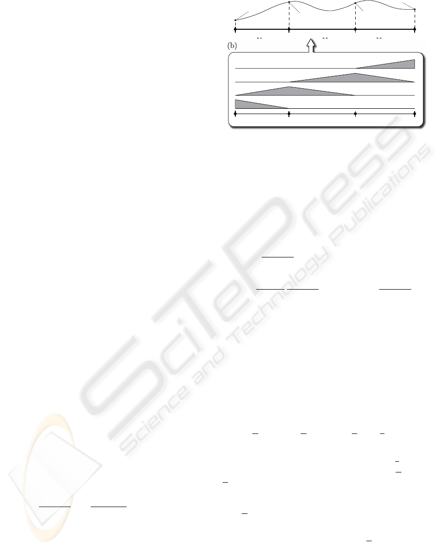
where Ψ
i
(z) are analytic functions called the shape
functions, e.g. see Fig. 2 (b), and N
dof
denotes the
degree of freedom of the resulting system description.
The essence of all spatial decomposition methods
such as the finite-difference, the finite-element, and
the finite-spectral method lies in the choice of the
shape functions Ψ
i
(z). This function is to be spec-
ified in more detail later.
Due to the fact that such approximated solution
cannot satisfy the partial differential equation (1)
everywhere in the region of interest a residual is left.
A common method known as the Galerkin formula-
tion is based on finding a way to make this resid-
ual small in some sense; achieved by minimizing
an appropriate number of weighted integrals. The
most popular choice for the weighting functions is
the shape function itself. Replacing both the solution
function f (z, t) and the input function s(z, t) by a fi-
nite expansion (4), denoted by
˜
f(z, t) and ˜s(z, t), re-
spectively, leads to following weighted integral over
the solution domain Ω
Z
Ω
Ψ
i
(z)
"
∂
˜
f(z, t)
∂t
− c
∂
2
˜
f(z, t)
∂z
2
− ˜s(z, t)
#
dz = 0
(5)
It can be stated that the minimization of this integral
automatically leads to the best numerical approxima-
tion of the solution f(z, t) of the partial differential
equation (Baker, 1983).
Then, the integral of (5) can be recasted by using
the rules of product differentiation. Applying the fun-
damental theorem of calculus for the evaluation of the
Ω
Ω
1
Ω
2
Ω
3
(b)
(a)
Ω
1
Ω
2
Ω
3
Global bases (shape functions)
0
1
0
1
z
0
z
1
z
2
z
3
Ψ
0
(z)
Ψ
1
(z)
Ψ
2
(z)
Ψ
3
(z)
z
1
z
2
z
3
f(z, t)
α
0
(t)
α
1
(t)
α
2
(t)
α
3
(t)
Figure 2: The solution f(z, t) of the partial differential
equation is approximated by
˜
f(z, t) depending on the shape
functions Ψ
j
(z) and their weighting coefficients α
j
(t). (a)
Elemental decomposition of the solution domain Ω into sev-
eral subdomains Ω
e
. (b) Shape functions Ψ
i
(z) for the lin-
ear case.
resulting integral leads to
Z
Ω
Ψ
i
(z)
∂
˜
f(z, t)
∂t
dz =
Z
Ω
Ψ
i
(z)˜s(z, t)dz (6)
− c
Z
Ω
dΨ
i
(z)
dz
∂
˜
f(z, t)
∂z
dz + c
"
Ψ
i
(z)
∂
˜
f(z, t)
∂z
#
∂Ω
r
∂Ω
l
where the last term on the right-hand side contains the
boundary conditions, i.e., ∂Ω
r
and ∂Ω
l
denotes the
right-hand and left-hand boundary, respectively. This
weighted residual statement is known as the weak for-
mulation of the partial differential equation (1).
As it is shown in the next sections, by specifying
the shape functions Ψ
i
(z) the weighted residual state-
ment (6) can be reduced to a system of ordinary dif-
ferential equations in α
i
(t), i.e., the semi-discrete ver-
sion of problem (1),
M
G
˙x(t) = M
G
u(t) − c D
G
x(t) + b
∗
(t) . (7)
In this system, M
G
is called the global mass matrix
and D
G
is the global diffusion matrix, and b
∗
repre-
sents the boundary conditions. The vector x(t) and
˙x(t) are the state vectors of the unknown weighting
coefficients α
i
(z) and their derivatives
x(t) =
α
0
(t), α
1
(t), · · · , α
N
dof
−1
(t)
T
.
It is important to note that the entries of the matrices
M
G
and D
G
, and the state vector x(t) merely de-
pend upon the choice of the shape functions Ψ
i
(z), as
shown in the following sections.
The next sections are devoted to appropriate def-
initions of the shape functions Ψ
i
(z). First, the h-
type expansion functions decomposing the solution
domain into small subdomains are considered; Ψ
i
(z)
ICINCO 2006 - SIGNAL PROCESSING, SYSTEMS MODELING AND CONTROL
18
are usually linear functions or simple polynomials.
Then, based on this decomposition it is possible to in-
troduce additional supporting nodes within the subdo-
mains; the so-called nodal p-type expansion functions
using higher-order orthogonal polynomials. Finally,
the shape functions Ψ
i
(z) can be defined by a set of
orthogonal polynomials of different order or modes,
called modal p-type expansion functions. For each
type it is shown that the global mass matrix M
G
and
the global diffusion matrix D
G
can be calculated in a
similar manner.
3.2 Elemental Decomposition
(h-type extension)
In this section, the decomposition of the solution do-
main Ω into small subdomains Ω
e
is demonstrated in
more detail, which is referred to as the h-type exten-
sion process. This process basically reduces the sizes
of the individual subdomains Ω
e
in order to achieve
convergence of the approximated solution.
Here, the decomposition process is explained and
visualized by means of simple polynomials for the
shape functions Ψ
i
(z). However, the same techniques
can be exploited with higher-order polynomial ex-
pressions, as shown in the next sections. The decom-
position of the solution domain into subdomains and
the respective shape functions for linear polynomials
are visualized in Fig. 2.
Substituting the finite expansion (4) into the weak
formulation (6) of the partial differential equation
yields the following individual terms of the weak for-
mulation
Z
Ω
Ψ
i
(z)
∂
˜
f(z, t)
∂t
dz =
N
dof
−1
X
j=0
M
g
ij
dα
j
(t)
dt
Z
Ω
dΨ
i
(z)
dz
∂
˜
f(z, t)
∂z
dz =
N
dof
−1
X
j=0
D
g
ij
α
j
(t)
Z
Ω
Ψ
i
(z)˜s(z, t)dz =
N
dof
−1
X
j=0
M
g
ij
ˆs
j
(t)
The individual entries M
g
ij
and D
g
ij
, defined by
M
g
ij
=
Z
Ω
Ψ
i
(z)Ψ
j
(z)dz ,
D
g
ij
=
Z
Ω
dΨ
i
(z)
dz
dΨ
j
(z)
dz
dz ,
can be assembled to the global mass matrix M
G
and
the global diffusion matrix D
G
, respectively. At this
point it can be easily recognized that this always leads
to the ordinary differential equation given in (7).
Furthermore, it is noted that in the case of linear
shape functions Ψ
i
(z) this leads to finite-difference
Ω
Ω
1
Ω
2
Ω
3
z = χ
e
(ξ)
(b)
(a)
(c)
z
0
z
1
z
2
z
3
Ω
1
Ω
2
Ω
3
Ψ
0
(z)Ψ
3
(z)Ψ
6
(z)Ψ
9
(z)
z
0
z
1
z
2
z
3
ξ
1
ξ
2
−1
0
1
0
1
0
1
0
1
1
ξ
1
ξ
2
−11
ξ
1
ξ
2
−11
ξ
1
ξ
2
−11
ψ
e
0
(ξ)
ψ
e
1
(ξ)
ψ
e
2
(ξ)
ψ
e
3
(ξ)
f(z, t)
α
1
(t)
α
2
(t)
α
3
(t)
α
7
(t)
α
9
(t)
Nodal expansion modes (global bases)
Nodal expansion modes (local bases)
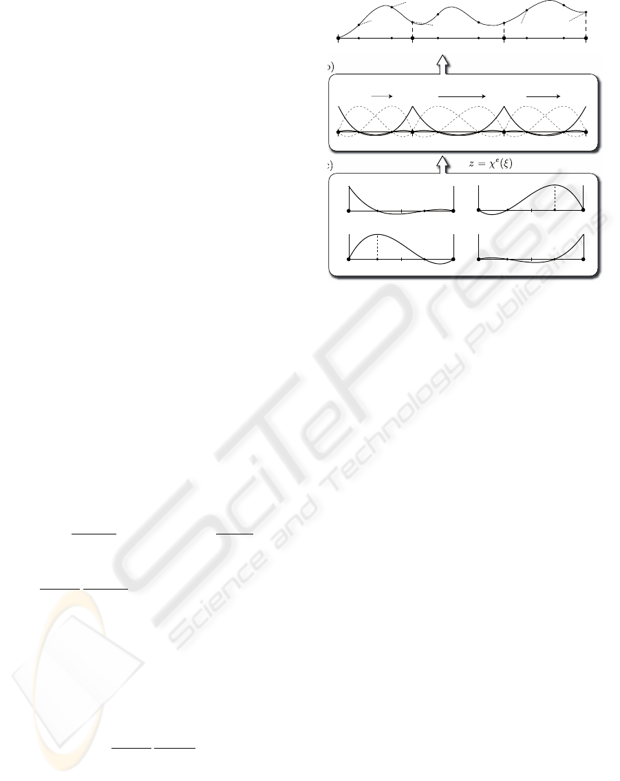
Figure 3: Approximation of the solution f(z, t) by means
of a nodal polynomial expansion, e.g. Legendre polynomi-
als for m = 4 refinement. (a) Elemental decomposition
of the solution domain Ω into several subdomains Ω
e
. (b)
Shape functions Ψ
i
(z) for a nodal polynomial expansion
visualized in global bases, and (c) in local bases (standar d
element).
formula, which can be regarded as a special case of
the finite-element method (Baker, 1983).
3.3 Nodal Polynomial Expansion
This section describes how the weak formulation (6)
is decomposed in space using higher order polynomi-
als; also called p-type expansion. Assuming a fixed
mesh, these methods achieve a higher accuracy of the
solution by increasing the polynomial order inside the
element.
Since a consideration of the expansion in terms of
global modes Ψ
i
(z) is uneconomical and numerically
intractable, especially when using a large number of
elements, it is reasonable to introduce a standard ele-
ment Ω
st
, such that
Ω
st
= {ξ | − 1 ≤ ξ ≤ 1} .
This standard element Ω
st
can be mapped to any el-
emental domain Ω
e
using the isoparametric transfor-
mation χ
e
(ξ), which expresses the global coordinate
z in terms of the local coordinate ξ, depicted in Fig. 3
(b)-(c).
A class of nodal p-type expansions which also have
become known as spectral elements are based on the
Legendre polynomials. Those polynomials are de-
BAYESIAN ESTIMATION OF DISTRIBUTED PHENOMENA USING DISCRETIZED REPRESENTATIONS OF
PARTIAL DIFFERENTIAL EQUATIONS
19
fined in the standard domain Ω
st
according to
L
m
(ξ) =
1
2
m
m!
d
m
(ξ
2
− 1)
m
dξ
m
,
where m denotes the degree of the used polynomial.
Based on the Legendre polynomials the spectral ele-
ments are given by
ψ
e
p
(ξ) =
(1 − ξ
2
)L
0
m
(ξ)
m(m + 1)L
m
(ξ
p
)(ξ
p
− ξ)
,
where L
m
is the Legendre polynomial of degree m,
L
0
m
denotes the differentiation with respect to the ar-
gument, and ξ
p
is the p-th Gauss-Lobatto-Legendre
quadrature point defined by the corresponding root of
(1 − ξ
2
) L
0
m
(ξ) = 0.
The choice of these quadrature point plays an im-
portant role in the stability of the approximation. The
spectral elements ψ
e
p
(ξ) are shown in the standard do-
main Ω
e
in Fig. (3) for m = 4, (Fournier et al., 2004).
Finally, considering the approximated solution in
terms of the spectral elements ψ
e
p
(ξ), we can express
the approximate solution
˜
f(z, t) in terms of ψ
e
p
(ξ) ac-
cording to
˜
f(z, t) =
N
dof
−1
X
j=0
Ψ
j
(z) α
j
(t) =
N
el
X
e=1
m
X
p=0
ψ
e
p
(ξ) α
e
p
(t)
(8)
where ψ
e
p
(ξ) = ψ
p
([χ
e
]
−1
(z)) contains the transfor-
mation from local bases to global bases in terms of the
parametric mapping χ
e
(ξ). The coefficients α
j
(t) in
this form have a physical interpretation in that they
represent the solution of the partial differential equa-
tion (1) at the nodal points x
j
. This fact is exploited
for the derivation of a simple measurement gain ma-
trix H
k
, i.e., it turns out that it is reasonable to put the
sensor nodes onto the polynomial nodes, see Sec. 4.2.
Upon substituting the nodal expansion (8) into the
weak formulation of the partial differential equation
(6) the entries of the local mass matrices M
e
ij
and lo-
cal diffusion matrices D
e
ij
can be derived as
M
e
ij
=
Z
1
−1
ψ
e
i
(ξ)ψ
e
j
(ξ)dξ ,
D
e
ij
=
Z
1
−1
dψ
e
i
(ξ)
dξ
dψ
e
j
(ξ)
dξ
dξ . (9)
Considering the boundary conditions at the elemental
nodes, e.g. z
1
and z
2
in Fig. 3, the local matrices M
e
ij
and D
e
ij
can be easily assembled to the global mass
matrix M
G
and global diffusion matrix D
G
. This is
an automatic procedure known as global assembly.
3.4 Modal Polynomial Expansions
For the construction of p-type expansions it is often
favorable to select a set of orthogonal functions (poly-
Ω
Ω
1
Ω
2
α
0
(t) ··· α
5
(t) α
5
(t) ··· α
10
(t)
(b)
(a)
(c)
Ω
1
Ω
2
Modal expansion modes (global bases)
z
0
z
1
z
2
Ψ
0
(z)
Ψ
5
(z)Ψ
10
(z)
z
0
z
1
z
2
f(z, t)
Modal expansion modes (lo cal bases)
ξ
−1
1
0
−1
1
0
−1
1
0
−1
1
0
ξ
ξ
ξ
ξ
ξ
ψ
e
0
(ξ)
ψ
e
1
(ξ)
ψ
e
2
(ξ)
ψ
e
3
(ξ)
ψ
e
4
(ξ)
ψ
e
5
(ξ)
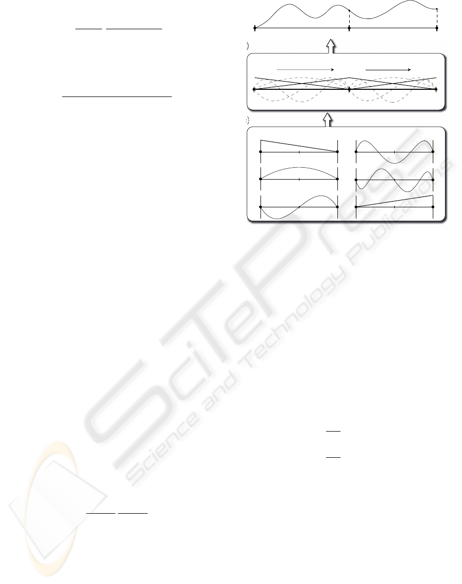
Figure 4: Approximation of the solution f(z, t) by means
of a modal polynomial expansion, e.g. Legendre polyno-
mials for m = 5 refinement. (a) Elemental decomposition
of the solution domain Ω into several subdomains Ω
e
. (b)
Shape functions Ψ
i
(z) for a modal polynomial expansion
visualized in global bases, and (c) in local bases (standar d
element).
nomials), such as Legendre, Chebyshev or sine func-
tions. The most commonly used orthogonal polyno-
mials in computational fluid dynamics, which offer
some advantages compare to the other polynomials,
are based upon the Legendre polynomials. This p-
type modal expansion modes in the standard element
Ω
st
are defined as
ψ
e
p
(ξ) =
1−ξ
2
p = 0
(1 − ξ
2
)L
0
p−1
(ξ) 0 < p < m
1−ξ
2
p = m
,
(10)
where the lowest expansion modes ψ
0
(ξ) and ψ
p
(ξ)
are the same as the linear finite element expansion.
These modes are denoted as boundary modes since
they are the only modes which are nonzero at the ends
of the interval. In Fig. 4 the p-type modal expansion
based upon the Legendre polynomials is depicted for
m = 5, (Karniadakis and Sherwin, 2005).
Thus, the approximate solution
˜
f(z, t) in terms
of a modal polynomial expansion can be expressed
in the same manner as the nodal polynomial expan-
sion (8); the function ψ
e
p
(ξ) is just replaced by p-
type modal expansion modes (10) and the coefficients
α
j
(t) denote the weighting coefficients for the indi-
vidiual modes.
The local mass matrices M
e
ij
and local diffusion
ICINCO 2006 - SIGNAL PROCESSING, SYSTEMS MODELING AND CONTROL
20

matrices D
e
ij
can be derived similar to the nodal poly-
nomial expansion (9). Considering the boundary con-
ditions at the end of each element, e.g. z
1
in Fig. 4,
the local matrices M
e
ij
and D
e
ij
can be easily assem-
bled to the global mass matrix M
G
and global diffu-
sion matrix D
G
.
4 TEMPORAL DISCRETIZATION
OF ODE-SYSTEM
In the previous section we presented the spatial de-
composition which allows the conversion of the par-
tial differential equation into a set of ordinary differ-
ential equation. In this section, we are now ready to
specifiy the time evolution leading to the discrete-time
system equation (2) and the discrete-time measure-
ment equation (3).
4.1 System Equation
To circumvent the restriction on the time step, ∆t,
it is reasonable to integrate the set of ordinary dif-
ferential equations (7) by means of implicit methods,
such as the Crank-Nicolson discretization. This pro-
duces a linear system of equations for the state vector
x
k+1
containing the unknown weighting factors α
i
at
the k + 1 time step, which is unconditionally stable.
Adding noise terms and modelling error terms leads
to following system equation
x
k+1
= A
k
x
k
+ B
k
u
k
+ b
k
+ w
k
, (11)
where the matrices A
k
and B
k
are determined using
the global mass matrix M
G
and the global diffusion
matrix D
G
. The vector b
k
containing the boundary
conditions is determined using the matrices M
G
, D
G
,
and the boundary vector b
∗
k
4.2 Measurement Equation
This section is devoted to the derivation of the
discrete-time measurement equation. The sensor
nodes, which are densely deployed inside the distrib-
uted phenomenon, are exploited to observe that phe-
nomenon and to improve its estimated state. That
means, the measurement of the i-th sensor node at the
location z = p
i
and at time step k, i.e., t = t
k
, is
related to the state vector x
k
according to
ˆy
i
(p
i
, t = t
k
) =
N
dof
−1
X
j=0
Ψ
j
(p
i
) α
j
(t = t
k
)
= Ψ
T
(p
i
) x
k
.
Assuming a sensor network consisting of L sensor
nodes, the measurement gain matrix H
k
is set up by
the shape function Ψ
T
(p
i
) of order N , according to
ˆy
k
=
Ψ
1
(p
1
) · · · Ψ
N
(p
1
)
.
.
.
.
.
.
.
.
.
Ψ
1
(p
L
) · · · Ψ
N
(p
L
)
| {z }
H
k
x
k
+ v
k
, (12)
where v
k
are the measurement uncertainties. The
number of rows L of the matrix H
k
depends on the
number of used sensors, i.e., number of measurement
points, and the number of columns N depends on the
desired number of modes.
However, in the case of nodal expansion and as-
suming that the sensors are located at the polynomial
nodes the weighting coefficients can be measured di-
rectly, i.e., α
j
(t) = ˆy
j
. In other words, the diagonal
entries of the measurement gain matrix H
k
are either
1 or 0, depending on the location of the sensor nodes,
ˆy
k
=
1 · · · 0
.
.
.
.
.
.
.
.
.
0 · · · 1
| {z }
H
k
x
k
+ v
k
. (13)
5 CENTRALIZED ESTIMATION
APPROACH
In this section the prediction step and the filter step for
a centralized estimation approach are derived. Due to
the fact that both the system equation (11) and the
measurement equation (3) are linear, it is sufficient
to use the linear Kalman filter to obtain the best pos-
sible estimate for the system state characterizing the
distributed phenomena.
5.1 Prediction Step
The purpose of the prediction step is to propagate the
current state estimate ˆx
e
k
through the system equation
(11) to the next time step. Thus, the mean of the pre-
dicted state vector ˆx
p
k+1
at time step k + 1 is given
by
ˆx
p
k+1
= A
k
ˆx
e
k
+ B
k
ˆu
k
+
ˆ
b
k
.
Assuming that the input vector u
k
and the state vector
x
k
are uncorrelated the covariance matrix is obviously
given by
C
p
k+1
= A
k
C
e
k
A
T
k
+ B
k
C
u
k
B
T
k
+ C
d
k
,
where C
u
k
is the covariance matrix of the input noise,
and C
d
k
is the covariance matrix of subsumed endoge-
nous uncertainties, e.g. modeling errors.
BAYESIAN ESTIMATION OF DISTRIBUTED PHENOMENA USING DISCRETIZED REPRESENTATIONS OF
PARTIAL DIFFERENTIAL EQUATIONS
21
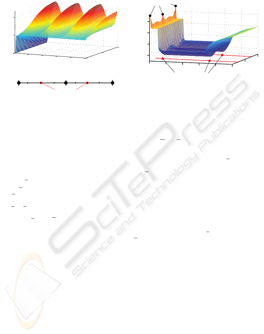
Ω
1
Ω
2
0 L
(b)
(a)
Sensors
2
4
8
time t
0
0
L
z
10
0
20
40
˜
f(z, t)
x
(1)
k
x
(3)
k
x
(5)
k
x
(7)
k
x
(9)
k
z
s1
z
s2
Figure 5: (a) Estimated solution
˜
f(z, t). (b) Elemental de-
composition into two elements Ω
1
and Ω
2
with a polyno-
mial expansion of order m = 5 and location of sensor
nodes.
5.2 Filter Step
For the purpose of reducing the estimation uncer-
tainty, measurements are used that are related to the
state via the measurement equation (3). Given the pre-
dicted state ˆx
p
k
with covariance C
p
k
and a vector ob-
servation ˆy
k
with covariance C
v
k
, the estimated state
vector ˆx
e
k
is derived by
ˆx
e
k
=ˆx
p
k
+ C
p
k
H
T
k
C
v
k
+ H
k
C
p
k
H
T
k
−1
·
ˆy
k
− H
k
ˆx
p
k
In the uncorrelated case the covariance matrix of the
estimate is given by
C
e
k
= C
p
k
− C
p
k
H
T
k
C
v
k
+ H
k
C
p
k
H
T
k
−1
H
k
C
p
k
.
6 SIMULATION RESULTS
In this section we demonstrate the performance of the
proposed estimation method by means of some simu-
lation results. The goal is the reconstruction of the
temperature distribution in a heat rod using both a
physical model and measurements obtained by a sen-
sor network. It is important to note that the novelty of
our approach is to consider the uncertainties arising
from noisy measurements and occuring in the physi-
cal model (state vector and input vector).
The evolution of the temperature is modelled by the
well-known one-dimensional heat equation (1) of a
bar with the length L = 1m. The noisy input func-
tion is given by s(z, t) = 30 sin(2 t) + 30 + ∆u
k
,
where ∆u
k
denotes the input uncertainties. Applying
Element nodes
Sensor: ON OFF
2
4
8
time t
0
−1
0
1
2
0
L
z
log(3σ )-Bounds
Figure 6: Logarithm of the 3σ-Bounds as a measure for
the uncertainty of the estimated solution
˜
f(z, t). Due to
the measurements the uncertainty can be decreased rapidly,
even between the sensor nodes.
a nodal expansion (8) for the approximated solution
˜
f(z, t) = Ψ
T
(z) α(t), the infinite-dimensional par-
tial differential equation (1) can be spatially and tem-
porally decomposed leading to the finite-dimensional
state space form (11). The state vector x
k
can be de-
rived by temporal discretization of the weighting fac-
tors α(t) of the approximated solution, as shown in
Sec. 4. Here, we assume a nodal expansion based on
a Legendre polynomial of the order m = 5. The spa-
tial decomposition of the heat rod into two elements
Ω
1
and Ω
2
is visualized in Fig. 5 (b).
Furthermore, it is assumed that for simplicity the
sensor network consists of two sensor nodes located
at z
s1
= 0.25 and z
s2
= 0.75, shown in Fig. 5 (b). In
the case of a nodal expansion the general relation be-
tween the measurement vector ˆy
k
and the state vector
x
k
described by (12) can be simplified to (13). For
this simulation example that means the state variables
x
(3)
k
and x
(7)
k
can be measured directly, as it is visual-
ized in Fig. 5 (b).
The estimated solution
˜
f(z, t) is visualized in Fig.
5 (a) and the logarithm of the 3σ-bound of the es-
timated solution
˜
f(z, t), which is a measure for its
uncertainty, is depicted in Fig. 6. It is obvious that
the measurements are used for rapidly decreasing the
uncertainty. Due to the model-based approach they
can be decreased even between the sensor nodes; the
remaining uncertainty merely arises from the model
uncertainties.
The estimation results for both a measurement
point and a non-measurement point are visualized in
Fig. 7. Again, it can be easily seen that the solution
˜
f(z, t) is estimated even at non-measurement points
with an appropriate certainty. Furthermore, it is clear
that by means of the measurements the estimated so-
lution
˜
f(z, t) can be significantly improved.
ICINCO 2006 - SIGNAL PROCESSING, SYSTEMS MODELING AND CONTROL
22
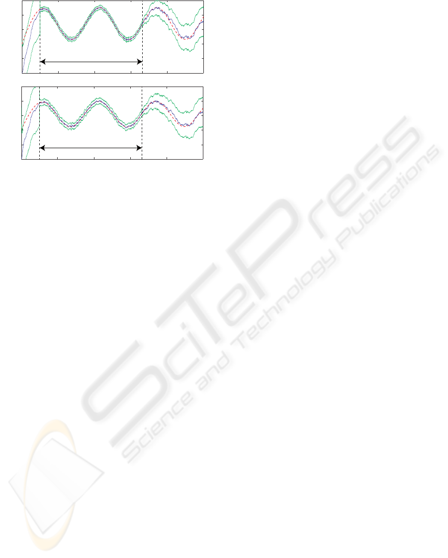
Sensor ON
Sensor ON
24 810time t
24 810time t
0
20
40
˜
f(z =0.25, t)
˜
f(z =0.5, t)
0
20
40
(b)
(a)
Figure 7: Estimated solution
˜
f(z, t) (blue), 3σ-Bounds
(green), and analytic solution f (z, t) (red) at (a) measure-
ment and (b) non-measurement point.
7 CONCLUSION
This paper introduced the methodology for deriv-
ing system models and measurement models for the
reconstruction of distributed phenomena character-
ized by means of linear partial differential equations.
Thanks to the inhomogeneous approximation capabil-
ities and the systematic manner of this approach, the
estimation of nonlinear phenomena even with com-
plex geometries is possible. The novelty of this paper
is the model-based reconstruction of distributed phe-
nomena under the consideration of uncertainties both
occuring in the physical model and arising from noisy
measurements.
It is believed that applying such methods in sensor
network applications for the reconstruction provides
novel prospects to optimal sensor node placement, op-
timal measurement time sequences, and improvement
of the used physical model. The performance of the
proposed model-based approach for the reconstruc-
tion of distributed pheonmena was demonstrated by
means of simulation results for the one-dimensional
partial differential equation.
Although for the one-dimensional partial differen-
tial equation, the decomposition may seem unneces-
sarily involved; however, the same principles can eas-
ily be applied to the decomposition in multiple dimen-
sions. This is left for future research work. Further-
more, especially for large sensor networks it is essen-
tial to find a decentralized reconstruction approach. It
is believed that the decomposition method introduced
in this paper is well-suited for such an estimation ap-
proach.
ACKNOWLEDGEMENTS
This work was partially supported by the German
Research Foundation (DFG) within the Research
Training Group GRK 1194 “Self-organizing Sensor-
Actuator-Networks”.
REFERENCES
Anderson, B. D. O. and Moore, J. B. (1979). Optimal Fil-
tering. Prentice-Hall.
Baker, A. J. (1983). Finite Element Computational Fluid
Mechanics. Taylor and Francis.
Culler, D. E. and Mulder, H. (2004). Smart sensors to net-
work the world. In Scientific American.
Faulds, A. L. and King, B. B. (2000). Sensor location in
feedback control of partial differential equation sys-
tems. In CCA’00, Proceedings of the 2000 IEEE In-
ternational Conference on Control Applications.
Fournier, A., Bunge, H.-P., Hollerbach, R., and Vilotte, J.-P.
(2004). Application of the spectral-element method to
the axisymmetric navier-stokes equation. In Geophys-
ical Journal International.
Hanebeck, U. D., Briechle, K., and Rauh, A. (2003). Pro-
gressive bayes: A new framework for nonlinear state
estimation. In Proceedings of SPIE, AeroSense Sym-
posium.
Karniadakis, G. E. and Sherwin, S. (2005). Spectral/hp
Element Methods for Computational Fluid Dynamics.
Oxford University Press.
Kumar, T., Zhao, F., and Shepherd, D. (2002). Collabora-
tive signal and information processing in microsensor
networks. In IEEE Signal Processing Magazine.
Levin, J. G., Iskandarani, M., and Haidvogel, D. B. (2000).
A nonconforming spectral element ocean model. In
International Journal for Numerical Methods in Flu-
ids.
Ortmaier, T., Groeger, M., Boehm, D. H., Falk, V., and
Hirzinger, G. (2005). Motion estimation in beating
heart surgery. In IEEE Transactions on Biomedical
Engineering.
Rao, B., Durrant-Whyte, H., and Sheen, J . (1993). A fully
decentralized multisensor system for tracking and sur-
veillance. In International Journal of Robotics Re-
search.
Roberts, K. and Hanebeck, U. D. (2005). Prediction and re-
construction of distributed dynamic phenomena char-
acterized by linear partial differential equations. In
Fusion’05, The Eight International Conference on In-
formation Fusion.
Thuraisingham, B. (2004). Secure sensor information man-
agement and mining. In IEEE Signal Processing Mag-
azine.
BAYESIAN ESTIMATION OF DISTRIBUTED PHENOMENA USING DISCRETIZED REPRESENTATIONS OF
PARTIAL DIFFERENTIAL EQUATIONS
23
