
Fast Algorithm for Optimal Polygonal Approximation of
Shape Boundaries
Prabhudev I. Hosur
1
and Rolando A. Carrasco
2
1
ClearCube Technology,
Austin, TX 78759, USA.
2
Department of Electrical, Electronic and Computer Engineering
University of Newcastle upon Tyne, UK.
Abstract. This paper presents fast optimal algorithm for approximation of a
shape boundary with a polygon having minimum number of vertices for a given
maximum tolerable approximation error. For this purpose, the directed acyclic
graph (DAG) formulation of the polygonal approximation problem is considered.
The reduction in computational complexity is achieved by reducing the num-
ber of admissible edges in the DAG and speeding up the process of determining
whether the edge distortion is within the tolerable limit. The proposed algorithm
is compared with other optimal algorithms in terms of the execution time.
1 Introduction
Representation of shape boundaries is of great interest in a number of fields such as
object-based video coding, video content retrieval based on object descriptions, object
recognition etc. The efficient way to represent shape boundaries is the polygonal ap-
proximation. The optimality of polygonal representation with respect to number of ver-
tices is relevant in applications involving pattern analysis, recognition, matching and
search and retrieval because in these applications, the speed of algorithms is propor-
tional to the number of vertices of the polygon.
The classical method for polygonal approximation is the iterative refinement method
(IRM) [1][2] in which a shape boundary is recursively split into polygon edges until the
maximum deviation between the boundary and the polygon lies below a predefined
error threshold. However, IRM is not the optimal solution because it does not always
yield the minimal number of polygon vertices. Several methods have been proposed for
polygonal approximation that provide strictly optimal solutions according to a certain
optimization criterion. A scan-along algorithm for optimum polygon approximation
of planar curves that yields the minimal number of edges is presented in [3]. A dy-
namic programming algorithm for optimal polygon approximation is presented in [4].
Recently in [5], the rate-distortion optimized polygonal approximation is obtained by
formulating the problem as finding the shortest path in a single source weighted directed
acyclic graph (DAG). The optimal approaches are in general computationally intensive
and are not suitable for real-time applications. Therefore, reducing the computational
complexity of optimal approaches is very important.
I. Hosur P. and A. Carrasco R. (2005).
Fast Algorithm for Optimal Polygonal Approximation of Shape Boundaries.
In Proceedings of the 5th International Workshop on Pattern Recognition in Information Systems, pages 104-113
DOI: 10.5220/0002579501040113
Copyright
c
SciTePress

In the DAG formulation of the optimal polygonal approximation problem, the com-
putational complexity can be decreased by reducing the number of edges in the DAG.
In the sliding window method proposed in [6], the number of edges in the DAG formu-
lation are reduced by considering only those edges from each vertex which lie within a
window of predefined size starting from that vertex. However, the ad-hoc window size
may yield sub-optimal results as demonstrated through our experimental results pre-
sented in Section 6. Another method for reducing the edges in the DAG formulation is
proposed in [7]. This method utilizes the fact that, as we scan-along a shape boundary,
there can no longer be any admissible edge beyond the boundary scan-point at which
the edge distortion exceeds twice the value of the error threshold.
This paper presents an algorithm for optimal polygonal approximation of shape
boundaries that yields significantly better speed-up performance as compared to other
optimal algorithms. The main idea of the proposed algorithm is to reduce the complexity
associated with the computation of edge distortion in addition to the reduction of the
number of edges.
The paper is organized as follows. Section 2 states the problem of optimal polygo-
nal approximation. The DAG formulation of the problem is introduced in Section 3. In
Section 4, the reference algorithms for optimal polygonal approximation are explained.
The proposed algorithm is described in Section 5. The performance of the proposed al-
gorithm is compared with that of the reference algorithms in Section 6. The conclusions
are given in Section 7.
2 Problem Statement
Suppose a shape boundary is represented by a closed digital contour denoted by the
ordered set C = {c
0
, c
1
, c
2
, . . . c
N
C
}, where c
0
= c
N
C
. Given C and an error threshold
δ, we are required to obtain a polygon P with minimal number of vertices such that
P ⊆ C and the maximal distance between P and C is less than or equal to δ. We
denote such a polygon by the ordered set P = {p
0
, p
1
, p
2
, . . . p
N
P
}. At this stage, it is
assumed that p
0
= c
0
.
Let
−−−−−→
p
k−1
, p
k
be the polygon edge that approximates the partial contour {c
i
=
p
k−1
, c
i+1
, ...c
i+L
= p
k
} containing (L + 1) points as shown in Fig. 1. The edge
distortion of
−−−−→
p
k−1
p
k
, denoted by d(p
k−1
− p
k
), is defined as the maximum distance
between
−−−−→
p
k−1
p
k
from the partial contour which it approximates. Mathematically,
d(p
k−1
, p
k
) = max
c
j
∈{c
i
=p
k−1
,c
i+1
,...c
i+1
=
p
k
}
d
′
(
p
k−1
,
p
k
,
c
j
) , (1)
where d
′
(p
k−1
, p
k
, c
j
) denotes the distance of the contour point c
j
from the edge
−−−−→
p
k−1
p
k
.
Let D(P ) denote the maximal distance of the polygon P from the contour C. We
can express D(P ) as the function of polygon edge distortions, as follows.
D(P ) = max
k∈{1,...
N
p
}
d (
p
k−1
,
p
k
) . (2)
105

c
j
c
i
p
k
p
k-1
c
i+L
d(p
k-1
, p
k
)
d'(p
k-1
, p
k
, c
j
)
Fig.1. Computation of edge distortion.
The optimization problem can be stated as,
min N
p
subject to
D(P ) ≤ δ (3)
3 Formulation of the problem in the form of directed acyclic graph
Let a weighted directed acyclic graph with the set of graph vertices V and the set of
graph edges E be denoted as G = (V, E). A directed graph edge is denoted by the
ordered pair (v
i
, v
j
) ∈ E, which implies that the edge starts at the vertex v
i
and ends
at vertex v
j
. Let the graph edge set E consist of every possible combination of (v
i
, v
j
)
such that i < j. The optimal polygonal approximation problem can be formulated using
a DAG such that the vertices and edges of the DAG correspond to possible vertices and
edges of the polygonal approximation, respectively. Consider a DAG with V = C such
that a directed graph edge (v
i
, v
j
) represents the polygon edge
−−→
c
i
c
j
. Furthermore, let
the weight w(v
i
, v
j
) of a graph edge (v
i
, v
j
) depend on the edge distortion d(c
i
, c
j
) of
the polygon edge
−−→
c
i
c
j
as follows.
w(v
i
, v
j
) =
(
∞, if d(c
i
, c
j
) > δ;
1, if d(c
i
, c
j
) ≤ δ.
(4)
An edge is called an admissible edge if its weight is equal to one; otherwise it is
called an inadmissible edge. The length of a path in this DAG becomes infinity if that
path includes an inadmissible edge (i.e., an edge corresponding to the polygon edge
106

distortion greater than δ). Therefore the DAG shortest path algorithm will not select
these paths. As a result, every path that starts at c
0
and ends at c
N
c
and has finite length
represents a valid polygonal approximation. Therefore, the shortest of all these paths
corresponds to the polygon approximation with smallest number of vertices, which is
the solution to the problem in (3).
4 Reference Algorithms
The conventional algorithm (CA) for the determination of the optimal polygon approx-
imation is through exhaustive search for the single source shortest path within the DAG
[5][7]. Let R
i
represent the minimum number of vertices that connect the initial ver-
tex v
0
to ith vertex v
i
in the DAG. The conventional optimal algorithm [7] is given as
follows.
R
0
= 0;
for (i = 1, . . . N
C
) {
R
i
= ∞
}
for (i = 0, . . . N
C
− 1) {
for (j = i + 1, . . . N
C
) {
calculate edge distortion d(c
i
, c
j
);
if (d(c
i
, c
j
) > δ) continue j;
if (R
i
+ 1 < R
j
)
{R
j
= R
i
+ 1; β
j
= i; }
}
}
After execution of the above algorithm, a (R
j
, β
j
) pair would have been stored at
each vertex position. The optimal polygon P = {p
0
= c
0
, p
1
, ...p
N
P
= c
N
C
} is then
obtained by tracing back the pointers starting from β
N
C
as follows.
N
P
= R
N
C
;
p
N
P
= c
N
C
;
k = N
C
;
for (i = N
P
, . . . 0) {
p
i−1
= c
β
k
k = β
k
}
The edge distortion d(c
i
, c
j
) of the edge connecting c
i
≡ (x
i
, y
i
) to c
j
≡ (x
j
, y
j
) is
computed using (1) as follows. Let c
k
≡ (x
k
, y
k
) be a boundary point between c
i
and
c
j
. The distance of c
k
from the edge
−−→
c
i
c
j
is given by [6],
d
′
(p
k−1
, p
k
, c
j
)
=
|(x
k
− x
i
)(y
j
− y
i
) − (y
k
− y
i
)(x
j
− x
i
)|
p
(x
i
− x
j
)
2
+ (y
i
− y
j
)
2
. (5)
107

The edge distortion d(c
i
, c
j
) is then computed as the maximum distance of the boundary
points that lie between c
i
and c
j
, from the edge
−−→
c
i
c
j
. If there are L boundary points
between the two end points of an edge, then L distances need to be computed using (5)
while determining the edge distortion of that edge. The conventional algorithm involves
the determination of
N
C
(N
C
−1)
2
number of edge distortions. Therefore, the conventional
algorithm is computationally intensive.
In [6], a sliding window is employed to reduce the numbers of edges in the DAG and
thereby reduce the total number of edge distortions that need to be computed. The main
idea is to restrict the number of admissible edges for each vertex within a window of
fixed length. The length of the window is predefined with an ad-hoc value; the smaller
the size of the window, the higher the speed-up. However, smaller window size may not
include all the admissible edges and therefore, it is less likely to yield optimal number
of vertices. The sliding window algorithm (SWA) provides improvement in speed at the
cost of being sub-optimal.
Another fast algorithm called Modified Schuster & Katsaggelos algorithm (MSK)
is presented in [7]. The main idea in this algorithm is to declare all the edges that lie
beyond the graph vertex at which the polygon edge distortion exceeds twice the error
threshold as inadmissible edges. This is equivalent to adapting the window size as we
scan along the graph based on the edge distortion observed at the current vertex.
5 Proposed Computationally Efficient Optimal Algorithm
The reference fast algorithms described in the previous section focus only on reducing
the number of edges in the DAG; thus, they do not reduce the complexity associated
with the computation of edge distortion to determine if that edge is a valid edge. In
order to achieve higher speed-up performance, we employ a different approach called
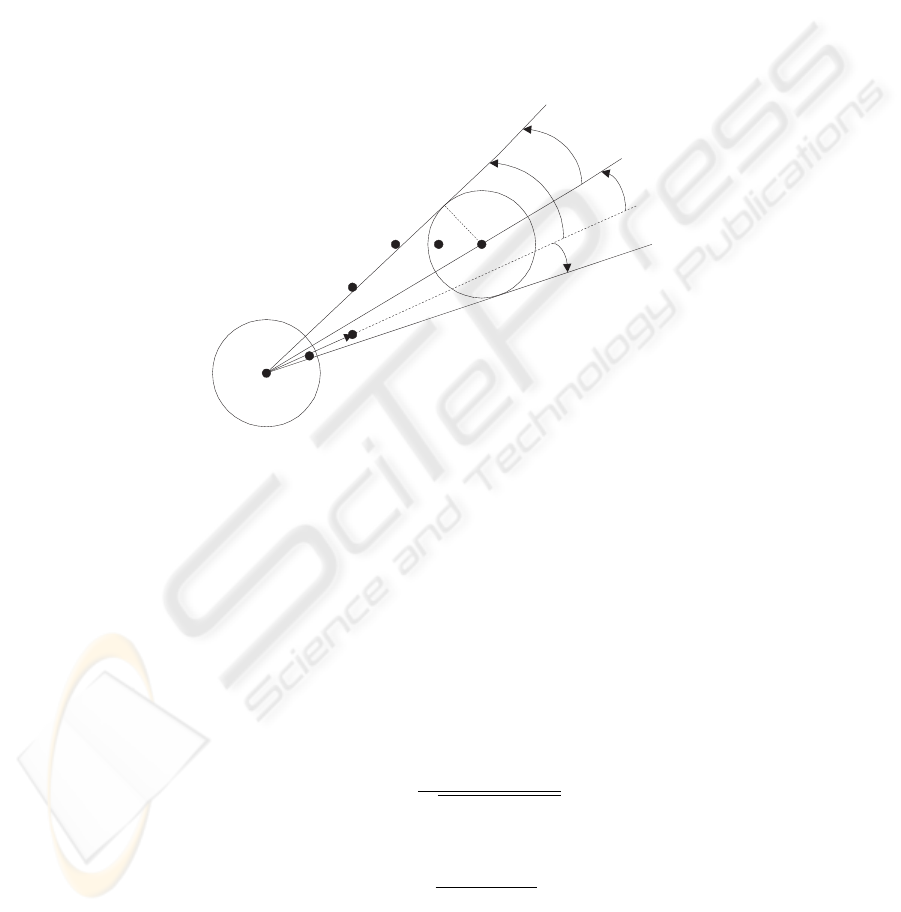
cone intersection method to the problem of determining whether an edge is a valid edge.
Suppose we wish to determine the set of all admissible edges starting from a vertex
c
i
. Consider the point c
i+1
. Let T
i+1
be the cone of straight lines formed by a disk of
radius δ centered at c
i+1
. The set of the straight lines from c
i
that lie within a distance
δ from c
i+1
are within the cone T
i+1
. Considering the next scan-point on the boundary,
c
i+2
, the set of the admissible straight lines from c
i
that lie within a distance δ from
both c
i+1
and c
i+2
are within the cone, T
i+1
T
T
i+2
. For a boundary point c
j
, the cone
of admissible straight lines that lie within a distance of δ from all the boundary points
in the current scan is S
j
= (T
i+1
T
T
i+2
. . .
T
T
j
). At each stage, we test if the current
boundary point c
j
lies within the cone S
j
. If the test succeeds, then the edge
−−→
c
i
c
j
is an
admissible edge; otherwise, it is an inadmissible edge.
Proposed Algorithm:
R
0
= 0;
for (i = 1, . . . N
C
) {
R
i
= ∞
}
for (i = 0, . . . N
C
− 1) {
108
for (j = i + 1, . . . N
C
) {
calculate the cone S
j
of admissible
straight lines;
if S
j
is empty, break j;
if
−−→
c
i
c
j
does not belong to S
j
continue j;
if (R
i
+ 1 < R
j
)
{R
j
= R
i
+ 1; β
j
= i; }
}
}
c
j
c
r
c
i
d
2
q
1
q
2
g
a
Fig.2. Illustration of cone intersection method.
We propose the following procedure to calculate the cone S
j
of admissible straight
lines starting from c
i
, and to test if
−−→
c
i
c
j
belongs to S
j
. The first step is to calculate
the angle of cone of straight lines shown in. Fig. 2. The angles are measured from a
reference vector
−−→
c
i
c
r
, where c
r
is the first point along the scan that lies at a distance
greater than δ from c
i
. The edges that lie before the reference vector are all admissible
edges.
Let c
i
≡ (x
i
, y
i
), c
r
≡ (x
r
, y
r
), and c
j
≡ (x
j
, y
j
). We define, (x
j
′
, y
j
′
) = (x
j
−
x
i
, y
j
− y
i
) and (x
′
r
, y
′
r
) = (x
r
− x
i
, y
r
− y
i
). From Fig. 2, we have,
γ
2
= arc tan
δ
q
x
′
j
2
+ y
′
j
2
− δ
2
!
(6)
α = arc tan
x
′
r
y
′
j
− y
′
r
x
′
j
x
′
r
x
′
j
+ y
′
r
y
′
j
!
(7)
109

(a) (b)
Fig.3. Original Boundaries: (a) Kid1 and (b) Kid2.
Since arc tan is in the principal range between −π/2 and π/2, the appropriate value of
α under special cases is calculated as follows. We add π to α to get new value of α if
any of the following are true: (a) α < 0 and (x
′
r
y
′
j
− y
′
r
x
′
j
) > 0 (this condition true if α
is in the 2nd quadrant), (b) α > 0 and (x
′
r
y
′
j
− y
′
r
x
′
j
) < 0 (this condition true if α is in
the 3rd quadrant). The angles θ
1
and θ
2
are calculated as follows.
θ
2
= α + γ
2
(8)
θ
1
= α − γ
2
(9)
The algorithm for determining the cone S
j
of admissible straight lines starting from c
i
,
and testing if
−−→
c
i
c
j
belongs to S
j
is given as follows.
S
i
= ∞;
if (j < r) {
S
j
= ∞;
−−→
c
i
c
j
∈ S
j
}
else {
T = [θ
1
, θ
2
];
S
j
= T
T
S
j−1
.
if (α ∈ S
j
)
(
−−→
c
i
c
j
∈ S
j
);
else (
−−→
c
i
c
j
/∈ S
j
);
}
6 Experimental Results
The proposed and the reference algorithms are evaluated using the shape boundaries
Kid1 and Kid2 consisting of 486 and 609 points, respectively. The shape boundaries are
shown in Fig. 3. The tolerable approximation error threshold δ is varied in steps from
110
0 1 2 3 4 5 6 7 8 9 10
0
200
400
600
800
1000
1200
1400
1600
1800
Tolerable error threshold (δ)
Speed−up with respect to the CA
Proposed
MSK
SWA (SW=5)
SWA (SW=20)
Fig.4. Comparison of speed-up of proposed optimal algorithm with other algorithms for Kid1.
0 to 10. Two separate tests are performed for MSK algorithm by setting window size
to 5 and 20. The execution times of each algorithm is obtained from the profiling in-
formation generated using the Rational’s Quantify (now part of IBM’s Purify) profiling
tool. The simulations are carried out on a desktop PC with 866 MHz Intel Pentium III
processor.
The execution time for CA changes by only negligibly small value when the value
of δ is varied. In our experiments, the execution time for CA is approximately 2751
milliseconds for Kid1 and 6086 milliseconds for Kid2. We compare the performance of
MSK, SWA and proposed algorithms for fast polygonal approximation with respect to
that of CA. The performance is measured in terms of number of polygonal vertices and
speed-up factor. Speed-up factor of a fast polygonal approximation algorithm is defined
as the ratio of the execution time of the conventional optimal algorithm (CA) to the that
of the fast algorithm.
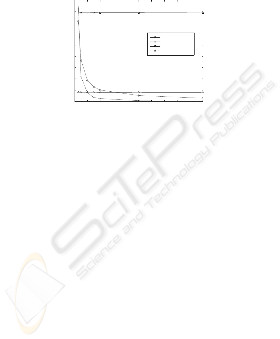
Fig. 4 and Fig. 5 show the comparison of speed-up performance of the proposed
algorithm with that of other fast algorithms for Kid1 and Kid2, respectively. Table 1
shows the number of vertices obtained with each algorithm. As compared to CA, the
proposed algorithm is more than 350 times faster at δ = 1 and more than 200 times
faster at δ = 2. In our experiments, the proposed algorithm is more than 2 times faster
than the MSK for δ > 0.3. For δ less than or equal to 0.3, the MSK is about 1.2
times faster than the proposed algorithm; this is because the number of edge distortion
computations in the MSK is small when the value of δ is very small. For SW=5, the
SWA is always faster than the proposed algorithm; but the results of SWA are always
sub-optimal (i.e., the number of vertices are more than those obtained with the optimal
algorithms) as shown in Table 1. For SW=20, the SWA is slower than the proposed
algorithm for lower values of δ and is faster for higher values of δ; again the results of
SWA are sub-optimal for δ ≥ 1.0 as shown in Table 1. Due to the fixed window size,
111
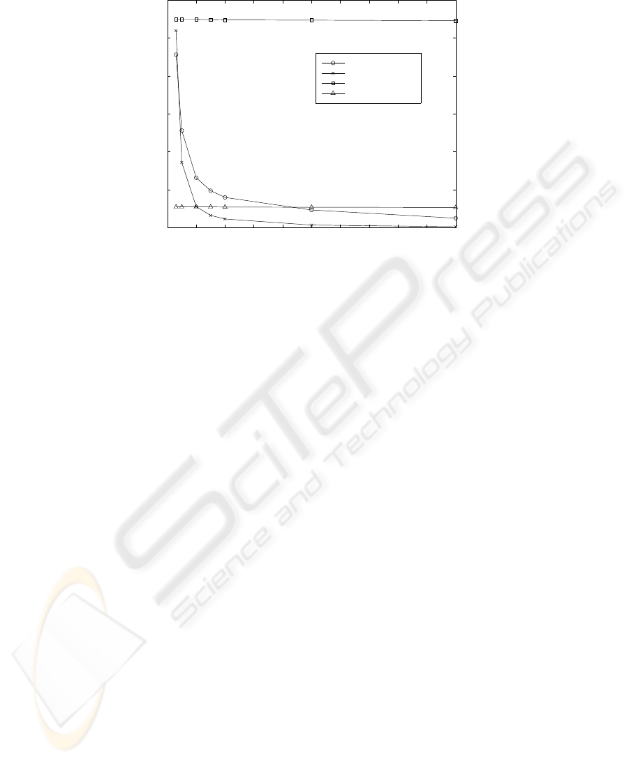
0 1 2 3 4 5 6 7 8 9 10
0
500
1000
1500
2000
2500
3000
Tolerable error threshold ( δ )
Speed−up with respect to the CA
Proposed
MSK
SWA (SW=5)
SWA (SW=20)
Fig.5. Comparison of speed-up of proposed optimal algorithm with other algorithms for Kid2.
the speed-up of SWA remains nearly the same for all values of δ. Whereas, the speed-up
of proposed and MSK algorithms decreases with increasing value of δ.
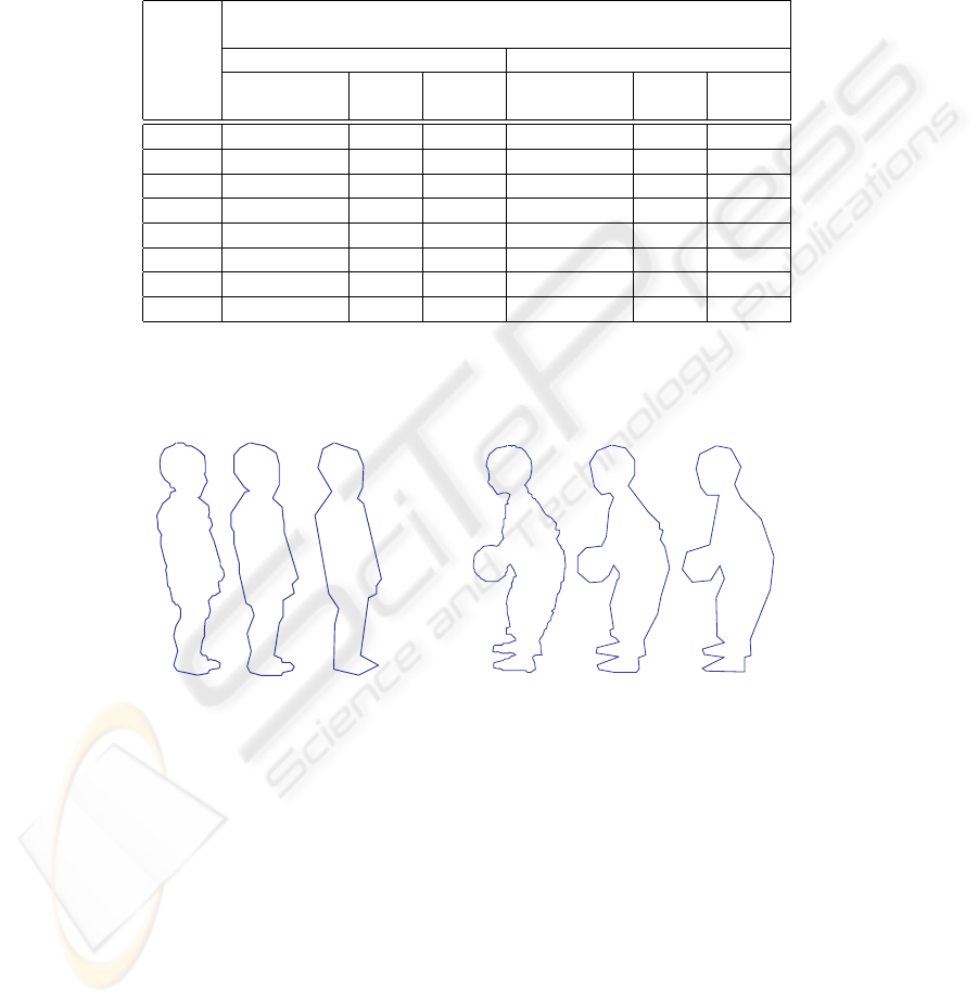
The polygon approximations of the boundaries obtained with the proposed algo-
rithm are shown in Fig. 6.
7 Conclusion
The proposed algorithm for optimal polygonal approximation is computationally very
efficient over a wide range of approximation error. On an average, it is about 450 times
faster than the conventional optimal algorithm and about 5 times faster than the MSK
algorithm [7]. Due to high speed-up performance, the proposed algorithm is suitable
for real-time shape representation and coding applications.
References
1. U. Ramer: An Iterative Procedure for the Polygon Approximation of Planar Curves. Computer
Graphics:Image Processing (1972)
2. MPEG: Description of Core Experiments on Shape Coding in MPEG-4 Video. ISO/IEC
JTC1/SC29/WG11 N1326 (1996)
3. J. G. Dunham: Optimum Uniform Piecewise Linear Approximation of Planar Curves. IEEE
Trans. Pattern Anal. Machine Intell. (1986)
4. J. C. Perez and E. Vidal: Optimum Polygonal Approximation of Digitized Curves. Pattern
Recognition Letters (1994)
5. G. M. Schuster and G. Melnikov and A. K. Katsaggelos: Operationally Optimal Vertex-Based
Shape Coding. IEEE Signal Processing Magazine (1998)
112
6. Katsaggelos A. K. et. al.: MPEG-4 Rate-Distortion-Based Shape-Coding Techniques. Pro-
ceedings of the IEEE (1998)
7. K. Schroder and P. Laurent: Efficient polygon approximations for shape signatures. Proceed-
ings of the IEEE International Conference on Image Processing (1999)
Table 1. Number of vertices in the polygonal approximation.
Tolerable Number of vertices in the
error polygonal approximation
threshold Kid1 Kid2
(δ) CA, MSK, SWA SWA CA, MSK, SWA SWA
Proposed Algo. ( SW=5) ( SW=20) Proposed Algo. ( SW=5) ( SW=20)
0 246 257 246 308 327 308
0.3 211 222 211 254 278 254
0.5 96 133 96 138 182 138
1.0 45 96 47 57 126 59
1.5 30 94 34 42 123 47
2.0 21 94 29 34 122 40
5.0 11 94 24 17 122 31
10.0 6 94 24 10 122 31
(a) (b) (c) (d) (e) (f)
Fig.6. Polygonal approximations using proposed optimal algorithm. (a)-(c): Kid1 at δ = 0.5,
δ = 1, and δ = 2, respectively. (d)-(f): Kid2 at δ = 0.5, δ = 1, and δ = 2, respectively.
113
