
A New Joinless Apriori Algorithm for Mining
Association Rules
Denis L. Nkweteyim and Stephen C. Hirtle
School of Information Sciences, 135 N. Bellefield Avenue, University of Pittsburgh,
Pittsburgh, PA 15260
Abstract: In this paper, we introduce a new approach to
implementing the
apriori algorithm in association rule mining. We show that by omitting the join
step in the classical apriori algoritm, and applying the apriori property to each
transaction in the transactions database, we get the same results. We use a
simulation study to compare the performances of the classical to the joinless
algorithm under varying conditions and draw the following conclusions: (1) the
joinless algorithm offers better space management; (2) the joinless apriori
algorithm is faster for small, but slower for large, average transaction widths.
We analyze the two algorithms to determine factors responsible for their
relative performances. The new approach is demonstrated with an application
to web mining of navigation sequences.
1 Introduction
Data mining aims to find useful patterns in large databases. Association rule mining is
a data mining technique that finds interesting correlations among a large set of data
items [1]. The mining results are presented as association rules—implications with
one or more items at the antecedent, and one or more at the consequent, of the rule.
Given a database D of transactions T, with each transaction comprising a set of items
(i.e., itemset), an association rule A⇒ B for the database is valid if A⊂T, B⊂T,
A∩B=φ, and A∪B and P(B/A) meet some minimum support and confidence
thresholds respectively.
The apriori algorithm [2, 3] has been influential in association rule mining (see for
exam
ple, [4-7]). The algorithm uses the apriori property – which states that all
nonempty subsets of a frequent itemset are also frequent – to reduce the search space
for determining candidate itemsets for inclusion in the rules set. The classical apriori
algorithm uses a join in each of n database scans to determine candidate itemsets for
inclusion in the rules set. Two main drawbacks to the algorithm are: (1) the number of
candidate itemsets generated by the join may be too big to fit into main memory, and
(2) high latency resulting from the need to scan the database during each iteration.
Tackling any of these problems is likely to lead to significant improvement on the
efficiency of the mining process.
In this paper, we introduce a new j
oinless apriori algorithm that significantly
reduces the search space required to determine frequent itemsets. The key difference
between this and the classical algorithm relates to the stage at which the apriori
L. Nkweteyim D. and C. Hirtle S. (2005).
A New Joinless Apriori Algorithm for Mining Association Rules.
In Proceedings of the 5th International Workshop on Pattern Recognition in Information Systems, pages 234-243
DOI: 10.5220/0002577802340243
Copyright
c
SciTePress

property is applied as the transaction database is scanned. In the kth iteration of the
classical algorithm, the apriori property is applied to the results of a join of frequent
(k-1)-itemsets to determine candidate k-itemsets, and the database scanned to
determine which of the candidate itemsets are frequent. In the joinless algorithm, the
join is eliminated: during the kth database scan the apriori property is applied to every
transaction with length l (l ≥ k) to determine candidate k-itemsets, and their support
counts incremented to enable determination of frequent k-itemsets at the end of the
iteration.
The rest of this paper includes:.differences between the two algorithms (Section
2); description of data and adaptation of the new algorithm to the data (Section 3); our
results and discussion (Section 4); and conclusions (Section 5).
2 The Classical and Joinless Apriori Algorithms
The classical apriori algorithm uses prior knowledge (the apriori property) of frequent
k-itemsets to prune the search space for the mining of (k+1)-itemsets. It begins by
finding frequent 1-itemsets L
1
, L
1
used to determine L
2
, L
2
used to determine L
3
, etc.
The generation of L
k
is a 2-step process comprising a join and a prune steps. The join
step determines frequent k-itemsets (L
k
) from frequent (k-1)-itemsets (L
k-1
) by joining
L
k-1
to itself. This results in k-itemsets to which the apriority property is applied, to
generate candidate k-itemsets (C
k
), which may or may not be frequent. The prune
step scans the transactions database to determine which of the candidate itemsets are
frequent; these are added to set L
k
.
The join step joins itemsets l
1
, l
2,
… l
k-1
of L
k-1
to each other, where two itemsets l
I
,
l
J
of L
k-1
are joinable if their first k-2 items are common (i.e., (l
I
[1] = l
J
[1])
∧
(l
I
[2] =
l
J
[2])
∧
…
∧
(l
I
[k-3] = l
J
[k-3])
∧
(l
I
[k-2] = l
J
[k-2])
∧
(l
I
[k-1] < l
J
[k-1]), where l
i
[j] is
the jth item in itemset l
i
). To illustrate the working of the classical apriori algorithm,
let the database D, of transactions be represented in Figure 1, and minimum support
count be 3. The steps required to generate frequent itemsets are illustrated in Figure
2. As can be seen from the figure, the algorithm iterates through the following steps:
• Determine candidate k-itemsets, C
k
• Scan the database to determine support count for each of the itemsets in C
k
• Compare the support count for each itemset in C
k
with minimum support count,
to determine frequent itemsets L
k
• Join L
k
to itself and apply the apriori property to determine C
k+1
Consider in greater detail, the application of the join and scan steps to determine
candidate itemsets and their support counts of. Consider for example, the join
between L
2
and itself, which generates an initial candidate 3-itemsets C
3
′
.
1. Join L
2
to itself , where L
2
= {{AB}{AC}{AE}{BC}{BE}}
• Initial candidate 3-itemsets C
3
′
: {{ABC}{ABE}{ACE}{BCE}}
2. Determine the 2-itemset subsequences:
• (ABC): {AB}{AC}{BC}
• (ABE): {AB}{AE}{BE}
235

• (ACE): {AC}{AE}{CE}
• (BCE): {BC}{BE}{CE
}
3. Use the apriori property to reject all members of C
3
′
that have one or more 2-
itemset subsequences that are not present in L
2
(i.e., in L
k-1
), i.e., whose support
counts are less than the minimum support count. This leaves candidate 3-itemset
subsequences C
3
= {{ABC}{ABE}}. In the example, CE does not have sufficient
support and is crossed out.
4. Determine if the itemsets in C
3
are frequent by scanning the database for all 3-
itemset subsequences and counting the number of occurrences of each C
3
itemsets.
• {ABC}: T001, T006, T007 (3 occurrences)
• {ABE}: T001, T007, T008 (3 occurrences)
We notice that both of the candidate 3-itemsets selected above meet the minimum
support count of 3 in this example, and so they are both included in L
3
.
The main benefit of the apriori property is the reduction in the number of candidate
itemsets, which leads to a reduction in both the space- and time-complexities of the
algorithm. But the number of candidate itemsets generated may still be too much to fit
into main memory. We now show how steps 1– 4 above are implemented using the
joinless apriori algorithm.
1. Scan the database for transactions involving 3 or more items, and determine an
initial candidate 3-itemsets C
3
′
.
• T001 (ABCE): {ABC}{ABE}{ACE}{BCE}
• T003 (ABD): {ABD}
• T006 (ABC): {ABC}
• T007 (ABCE): {ABC}{ABE}{ACE}{BCE}
• T008 (ABE): {ABE}
TID Items TID Items TID Items TID Items
T001 A,B,C,E T003 A,B,D T005 B,C T007 A,B,C,E
T002 B,C T004 A,C T006 A,B,C T008 A,B,E
Fig. 1. Sample transactions data used to show the working of the classical and joinless apriori
algorithms
236
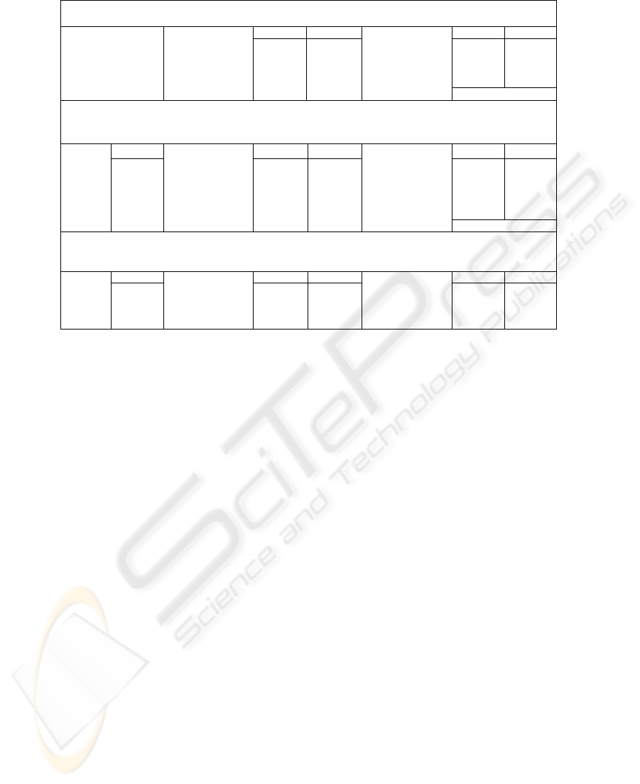
Step 1a: Scan database D for count of each candidate 1-itemset C
1
Step 1b: Compare C
1
itemsets with minimum support & generate L
1
C
1
Itemset Su
pp
ort
L
1
Itemset Su
pp
ort
{
A
}
6
{
A
}
6
{
B
}
7
{
B
}
7
{
C
}
6
{
C
}
6
{
D
}
1
Compare C
1
support count with
minimum support
{
E
}
3
Scan D to get
candidate 1-itemset
counts
{
E
}
3
Step 2a: Join L
1
to itself and use the Apriori property to generate candidate 2-itemsets C
2
Step 2b: Scan database D for count of each C
2
Step 2c: Compare C
2
itemsets with minimum support & generate L
2
Itemset C
2
itemset Support
L
2
Support
{
A
,
B
}
{
A
,
B
}
5
{
A
,
B
}
5
{
A
,
C
}
{
A
,
C
}
4
{
A
,
C
}
4
{
A
,
E
}
{
A
,
E
}
3
{
A
,
E
}
3
{
B
,
C
}
{
B
,
C
}
5
{
B
,
C
}
5
{
B
,
E
}
{
B
,
E
}
3
{
B
,
E
}
3
Join(L
1
L
1
) &
apply
Apriori
{
C
,
E
}
Scan D to get
candidate 2-itemset
counts
{
C
,
E
}
2
Compare C
2
support count with
minimum support
Step 3a: Join L
2
to itself and use the Apriori property to generate candidate 2-itemsets C
3
Step 3b: Scan database D for count of each C
3
Step 3c: Compare C
3
itemsets with minimum support & generate L
3
Itemset C
3
Itemset Su
pp
ort
L
3
Itemset Su
pp
ort
{
A
,
B
,
C
}
{
A
,
B
,
C
}
3
{
A
,
B
,
C
}
3
Join(L
2
L
2
) &
apply
Apriori
{A,B,E}
Scan D to get
candidate 3-itemset
counts
{A,B,E} 3
Compare C
3
support count with
minimum support
{A,B,E} 3
Fig. 2. The mechanics of the classical apriori algorithm applied to the database in Figure 1
2. Determine all the 2-itemset subsequences of the C
3
′
• T001 (A,B,C): {AB}{AC}{BC}
• T001 (A,B,E): {AB}{AE}{BE}
• T001 (A,C,E): {AC}{AE}{CE}
• T001 (B,C,E): {BC}{BE}{CE}
• T003 (A,B,D): {AB}{AD}{BD}
• T006 (A,B,C): {AB}{AC}{BC}
• T007 (A,B,C): {AB}{AC}{BC}
• T007 (A,B,E): {AB}{AE}{BE}
• T007 (A,C,E): {AC}{AE}{CE}
• T007 (B,C,E): {BC}{BE}{CE}
• T008 (A,B,E): {AB}{AE}{BE}
3. Use the apriori property to reject all 3-itemsets with one or more 2-itemset
subsequences that do not appear in L2 (i.e., Lk-1), i.e., whose support counts are
less than the minimum support count (recall L2 = {{AB}{AC}{AE}{BC}{BE}}).
In the example, CE and BD do not have support and are crossed out.
4. Count the occurrences of each 3-itemset subsequences that are not rejected in the
previous step to get their support counts. In this example, both {ABC} and {ABE}
meet minimum the support count of 3, and so are added to L
3
.
We note that the absence of the join step leads to better space complexity in the
joinless algorithm, especially for large transactions databases. This is because the
apriori property is applied to individual transactions, which usually involve much
fewer items than the database has transactions. Figure 3 summarizes the steps
237

involved in finding frequent itemsets for the database of Figure 1 using the joinless
apriori algorithm. Figure 4 presents the joinless apriori algorithm.
3 Data and Simulation
Our presentation of both the classical and joinless apriori algorithms so far has
assumed that the objective is to find association rules that describe the correlations
among all items in the transaction database. But there are situations where the mining
objective is to find the relationships between items in a transaction and only one or a
few other items in the transaction. In our research for example, we are interested in
finding the relationship between user navigation behaviors in hypermedia (as
evidenced by a set of navigation pages they visit, which form the antecedents of
mined association rules), and the Web pages they are presumed to be interested in
(i.e., content pages, which form the rule consequents). This information gives us the
basis for building models for making Web page recommendations to users. For the
rest of this paper, we refer to a database with well-defined consequents (or content
pages) as c-annotated (i.e., consequent-annotated). [8-12] discuss the classification of
Web pages into navigation and content pages.
The procedure to obtain frequent itemsets for a c-annotated transactions database
is identical to the case for a general transactions database, except that: (1) one of the
items in each transaction is annotated as the consequent of the association rules for
that transaction, and (2) candidate and frequent itemsets are generated only for the
non-annotated items of the transactions. For example, Figure 5 shows a c-annotated
transactions database, and Figure 6, the process of obtaining frequent itemsets for the
database.
For the purpose of analyzing the performance of the joinless apriori algorithm, we
used web server logs, but it should be emphasized that the source of the data is
immaterial to the performance of the algorithm. The data comprised the user access
log for the web site of the School of Information Sciences, University of Pittsburgh
for the months of June to August 2004. The raw data were collected in the common
log format [13] and totaled about 500MB.
We followed the heuristics presented in [8, 9, 12, 14, 15] to extract user sessions
from the server logs, and the maximal forward reference (MFR) heuristic [15] to
extract transactions within user sessions, with a transaction comprising one or more
navigation pages and terminating with a content page. In order to reduce the lengths
of very long transactions, we applied a new heuristic we are researching on. This
heuristic PR × ILW (page rank
×
inverse links to word count ratio) combines the page
rank algorithm [16, 17] and the links:word count ratio of web pages to classify them
as navigation or content pages. The distribution of transactions lengths obtained is
shown in Table 1.
Finally, we ran both the classical and joinless apriori algorithms on the
transactions database for the following values of minimum support count: 1, 2, 3, 12,
24, 59, 118, and 235 (corresponding to the following fractions of the transaction
database size: 0.000001, 0.000005, 0.00001, 0.00005, 0.0001, 0.00025, 0.0005,
0.001), and for different average association rule lengths. Average rule lengths were
controlled by varying the maximum acceptable transaction length L
max
between 5 and
238
10. For each run, all transactions whose lengths were larger than L
max
were ignored.
For the rest of this paper, we use the notation R
n,s
to refer to a run with L
max
set to n
and minimum support count set to s. All the simulations were run on a SunBlade 2500
workstation running the Sun Solaris 9 UNIX operating system. The programs were all
written in ANSI C, and compiled using the C compiler that comes with the operating
system.
Table 1. Distribution of transaction lengths using (MFR) and a combination of MFR and a
PR × ILW threshold of 5
Transaction
Lengths
2 3 4 5 6 7 8 9 10
11-
15
16-
20
21-
25
26-
30
31-
40
41-
50
51-
75
76-
100
101-
150
151-
200
Transaction
Count
Mean
Length
MFR
Count
12041 7461 4296 2805 1806 1341 868 615 536 1363 678 510 587 804 551 909 359 222 114 37866 9.53
MFR +
PR × ILW
Count
180377 34203 11183 4926 2735 492 226 155 118 234 106 78 51 58 33 4 0 0 0 234979 2.42
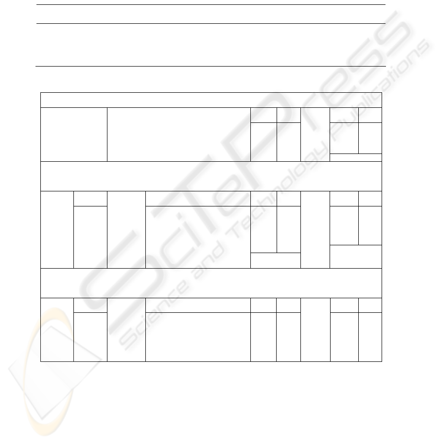
Step 1a: Scan database D for count of each candidate 1-itemset C
1
Step 1b: Compare C
1
itemsets with minimum support & generate L
1
C
1
Itemset
Support L
1
Itemset Support
{A} 6 {A} 6
{B} 7 {B} 7
{C} 6 {C} 6
{D} 1 {E} 3
Scan D to get candidate 1-itemset counts
{E} 3
Compare
C
1
support
count
with
minimum
support
Step 2a: Scan database D for transactions >= 2
Step 2b: Determine 2-itemset subsequences and apply Apriori property to get C
2
Step 2c: Count each subsequence to determine support count for C
2
Step 2d: Compare C
2
itemsets with minimum support & generate L
2
Transaction C
2
Itemsets
C
2
Itemset
Support
L
2
Itemset
Support
{A,B,C,E} {A,B}{A,C}{A,E}{B,C}{B,E}{C,E} {A,B} 5 {A,B} 5
{B,C} {B,C} {A,C} 4 {A,C} 4
{A,B,D} {A,B} {A,E} 3 {A,E} 3
{A,C} {A,C} {B,C} 5 {B,C} 5
{B,C} {B,C} {B,E} 3 {B,E} 3
{A,B,C} {A,B}{A,C}{B,C} {C,E} 2
{A,B,C,E} {A,B}{A,C}{A,E}{B,C}{B,E}{C,E}
Scan D for
transactions
w
ith 2 or
more items
{A,B,E}
Candidate 2-
itemset = 2-
itemset
subsequences
+ Apriori
{A,B}{A,E}{B,E}
Compare
C
2
support
count
with
minimum
support
Step 3a: Scan database D for transactions >= 3
Step 3b: Determine 3-itemset subsequences and apply Apriori property to get C
3
Step 3c: Count each subsequence to determine support count for C
3
Step 3d: Compare C
3
itemsets with minimum support & generate L
3
Transaction C
3
Itemsets
C
3
Itemset
Support
L
3
Itemset
Support
{A,B,C,E} {A,B,C}{A,B,E} {A,B,C} 3 {A,B,C} 3
{A,B,D} {A,B,E}
3
{A,B,E}
3
{A,B,C} {A,B,C}
{A,B,C,E} {A,B,C}{A,B,E}
Scan D for
transactions
w
ith 3 or
more items
{A,B,E}
Candidate 3-
itemset = 3-
itemset
subsequences
+ Apriori
{A,B,E}
Compare
C
3
support
count with
minimum
support
Fig. 3. The mechanics of the joinless apriori algorithm applied to the database in Figure 1
239
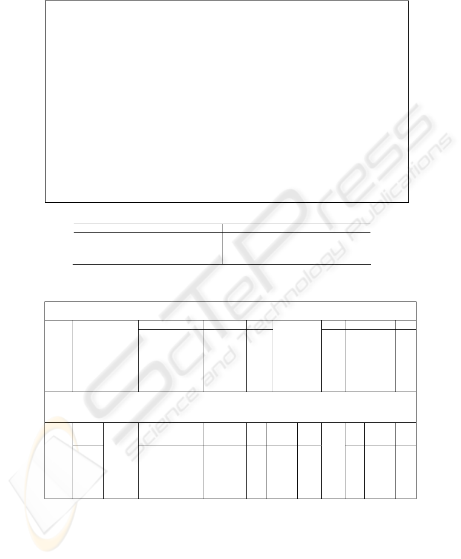
Fig. 4. The joinless apriori algorithm
TID Transaction Items Rule Consequent TID Transaction Items Rule Consequent
T001
A,B,C E T005 B C
T002
B C T006 A,B C
T003
A,B D T007 A,B,C E
T004
A C T008 A,B E
Fig. 5. C-annotated transactions database used to illustrate the working of the joinless apriori
algorithm
Step 1a: Scan database D transactions for count of each candidate 1-itemset C
1
Step 1b: Compare C
1
itemsets with minimum support & generate L
1
C
1
Itemset Consequent Support
L
1
It t
Consequent Support
{A} C 2 {B} C 3
{B} C 3 {A} E 3
{A} D 1 {B} E 3
{B} D 1
{A} E 3
{B} E 3
Scan D to get candidate
1-itemset counts
{C} E 2
Compare C
1
support with min.
support
Step 2a: Scan database D transactions for transactions >= 2
Step 2b: Determine 2-itemset subsequences and apply Apriori property to get C
2
Step 2c: Count each subsequence to determine support count for C
2
Step 2d: Compare C
2
itemsets with minimum support & generate L
2
Transaction C
2
Itemsets Consequent
C
2
Itemset
Consequent Support
L
2
Itemset
Consequent Support
{A,B,C} {A,B}{A,C}{B,C} E {A,B}
E 3
{A,B} E
3
{A,B} {A,B} D {A,C}
E 2
{A,B} {A,B} C {B,C}
E 2
{A,B,C} {A,B}{A,C}{B,C} E {A,B}
D 1
{A,B} {A,B} E {A,B}
C 1
Scan D for
trans. with
2 or more
items
Candidate 2-
itemset = 2-
itemset
subsequences
+ Apriori
Compare
C
2
support
with
min.
support
joinless apriori
{
L
1
= find_frequent_1-itemsets(D);
for (k = 2; L
k-1
≠ ∅; k++) {
/*scan D for transactions ≥ k*/
for each transaction t
∈
D | t.itemcount
≥
k
C
*
= subseq(t,k);
k
C
k
= joinless_apriori(L
k-1
, C
*
k
, min_sup);
L
= {c ∈ C
k
⎟ c.count
≥
min_sup}
k
}
return L = ∪
k
L
k
}
procedure joinless_apriori(L
: frequent (k-1)-itemsets; C
*
:
k-1
k
list of k-itemsets in D min_sup: min. support threshold) {
for each itemset c ∈ C
*
{
k
if has_infrequent_subset(c, L ) then
k-1
delete c; /*prune step; remove unfruitful candidate*/
else
add c to C
k
;
}
return C
k
}
procedure has_infrequent_subset(c:potential candidate k-itemset; L
k-1
:frequent (k-
1)-itemsets) {
for each (k-1)-subsets s of c
if s ∉ L
then /*apriori property*/
k-1
return TRUE
return FALSE
}
Fig. 6. The mechanics of the joinless apriori algorithm applied to the c-annotated database in
Figure 5
240
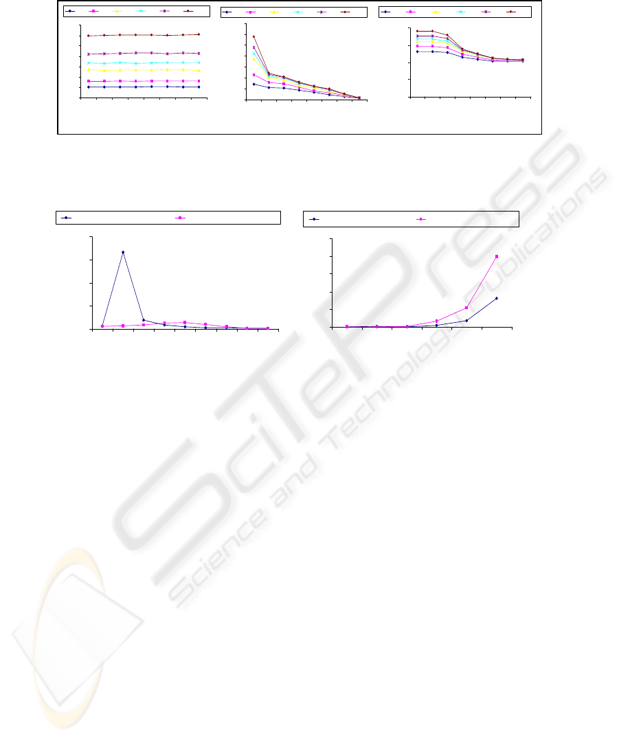
Fig. 7. Variation of execution time with minimum support count for (a) joinless apriori
algorithm and (b) classical apriori algorithm. (c) Variation of corresponding average rule length
with minimum support count
0
10
20
30
40
50
60
70
1 2 3 12 24 59 118 235
Minimum support count
Execution time (s)
R5,s
R6,s
R7,s
R8,s
R9,s
R10,s
0
100
200
300
400
500
600
700
1 2 3 12 24 59 118 235
Minimum support count
Execution time (s)
R5,s
R6,s
R7,s
R8,s
R9,s
R10,s
0
0.5
1
1.5
2
1 2 3 12 24 59 118 235
Minimum support count
Mean rule antecedent
length
R5,s
R6,s
R7,s
R8,s
R9,s
R10,s
0
1
2
3
4
5
123456
Rule antecedent length
Tim e per rule (s
)
Joinless Apriori Algorithm
Classical Apriori Algorithm
0
50
100
150
200
123456789
Rule antecedent length
Tot. time (s)
Classical Apriori Algorithm
Joniless Apriori Algorithm
c
a
b
Fig. 9. Variation of average rule
generation time with rule length for
R
10
,
12
Fig. 7. Variation of execution time with
rule length for R
9
,
59
4 Results and Discussion
Figures 7 shows the distribution of execution time and minimum support count for the
joinless and classical apriori algorithms ((a) and (b)), and the corresponding variation
in average rule length (c), with minimum support count. Figure 8 shows the typical
variation of average execution time per rule and the rule length. Figure 9 shows the
typical variation of total execution time as a function of rule length for the joinless
and classical apriori algorithms.
Figures 7 (a), (b), and (c) show that for both algorithms, execution time increases
with mean rule length; this is expected. In the joinless algorithm however, execution
time is fairly constant. Intuitively, one would expect the execution time to decrease
with increase in the minimum support count (as is the case with the classical
algorithm), since larger support thresholds translate to fewer rules generated. We also
see from Figures 7 (a) and (b) that the joinless apriori algorithm performs better than
the classical algorithm for small values of minimum support count (when a large
number of rules are generated), but the classical algorithm performs better for large
values of support threshold. The reason for this is related to the importance of the join
241

step in the classical algorithm: the smaller the number of rules generated, the smaller
the size of the tables resulting from the join, and the better the performance.
Figure 8 shows that for both the joinless and classical apriori algorithms, the time
used to generate a single rule increases exponentially with rule length. Both
algorithms do not suffer from an explosion of computational time for longer rules
however, since the number of these expensive, longer rules is much smaller.
Figure 9 illustrates the relative time efficiencies of both algorithms for different
rule lengths. The classical algorithm performs much worse than the joinless
algorithm for small rule lengths, while the joinless algorithm performs worse for
longer rules. The shape of the classical apriori algorithm curve can be explained as
follows: the first pass is inexpensive, involving only a count of 1-itemsets; the second
pass is very expensive as it involves a join; subsequent passes get less expensive
because the apriori property prunes the input to the join, reducing its cost.
5 Conclusion
In this paper, we have demonstrated a new implementation of the apriori property that
avoids the join step in the classical algorithm that is very expensive in terms of
memory use. This problem is insignificant in the joinless algorithm where the space
requirement is a function of the average transaction record size, which is typically
much smaller than the database size. Our algorithm also outperforms the classical
algorithm for smaller values of minimum support count.
References
1. Agrawal, R., Imielinski, T., Swami, A.: Mining Association Rules Between Sets of Items in
Large Databases. Proc. ACM SIGMOD Int. Conf. on Management of Data. ACM Press,
New York (1993) 207–216.
2. Aggarwal, C., Srikant, R.: Fast Algorithms for Mining Association Rules. Proc. 20th Int.
Conf. on Very Large Data Bases, VLDB. Morgan Kaufmann Publishers Inc., San Francisco
(1994) 487–499.
3 Mannila, H., Toivonen, H., Verkamo, I.: Efficient Algorithms for Discovering Association
Rules. AAAI Workshop on Knowledge Discovery in Databases (KDD-94), Seattle, WA
(1994) 181–192.
4 Han J., Kamber M.: Data Mining: Concepts and Techniques. Academic Press, San Diego,
CA, (2001)
5 Bodon, F., A fast APRIORI implementation. In Proceedings of the IEEE ICDM Workshop
on Frequent Itemset Mining Implementations, Melbourne, FL (2003)
6. Borgelt, C.: Efficient Implementations of Apriori and Eclat. In Proceedings of the IEEE
ICDM Workshop on Frequent Itemset Mining Implementations, Melbourne, FL (2003)
7. Kosters, W.A. and W. Pijls, Apriori, A Depth First Implementation. In Proceedings of the
IEEE ICDM Workshop on Frequent Itemset Mining Implementations, Melbourne, FL
(2003)
8 Cooley, R., Mobasher, B., and Srivastava, J.: Web Mining: Information and Pattern
Discovery on the World Wide Web. International Conference on Tools With Artificial
Intelligence, Newport Beach, CA (1997) 558–567.
242

9 Cooley, R., Mobasher, B., and Srivastava, J.: Data Preparation for Mining World Web
Browsing Patterns. Journal of Knowledge and Information Systems (1999) 5–32
10 Mobasher, B., Cooley, R., and Srivastava, J.: Automatic Personalization Based on Web
Usage Mining. Communications of the ACM, ACM Press (2000) 142–151
11 Mobasher, B., Dai, D., Luo, L., and Nakagawa, M.: Effective Personalization Based on
Association Rule Discovery from Web Usage Data. Proc. Third Int. Workshop on Web
Information and Data Management, ACM Press, New York (2001) 9–15
12 Pitkow, J.: In Search of Reliable Usage Data on the WWW. Proc. of the Sixth International
WWW Conference (1997)
13 W3C: The Common Logfile Format. Retrieved April 5 2003 from
http://www.w3.org/Daemon/User/Config/Logging.html
14 Pirolli, P.: Computational Models of Information Scent-following in a Very Large
Browsable Text Collection. Proc.SIGCHI Conf. on Human Factors in Computing Systems,
ACM, Atlanta, GA (1997)
15 Chen, M.S., Park, J.S., and Yu, P.S.: Data Mining for Path Traversal Patterns in a Web
Environment. Proc. of the 16th International Conference on Distributed Computing Systems
(1996) 385–392
16 Craven, P.: Google's PageRank Explained and How to Make the Most of it. Retrieved
September 5 2003 from http://www. webworkshop.net/pagerank.html.
17 Rogers, I.: The Google Pagerank Algorithm and How it Works. Retrieved September 5 2003
from http://www.iprcom.com/ papers/pagerank/.
243

244
