
Activity Identification and Visualization
1
Richard J. Parker
1
, William A. Hoff
2
, Alan Norton
3
,
Jae Young Lee
2
and Michael Colagrosso
2
1
Southwest Research Institute, San Antonio, Texas 78228
2
Colorado School of Mines, Golden, Colorado 80401
3
National Center for Atmospheric Research, Boulder, Colorado 80307
Abstract.
Understanding activity from observing the motion of agents is simple
for people to do, yet the procedure is difficult to codify. It is impossible to
enumerate all possible motion patterns which could occur, or to dictate the ex-
plicit behavioural meaning of each motion. We develop visualization tools to
assist a human user in labelling detected behaviours and identifying useful at-
tributes. We also apply machine learning to the classification of motion into
motion and behavioural labels. Issues include feature selection and classifier
performance.
1 Introduction
Surveillance observations are becoming increasingly available, meaning the ability to
continuously watch an area for long periods of time with multiple sensors. The types
of analysis required for today’s military (such as counter-terrorism) and commercial
security applications increasingly involve interpreting observations made over time.
The amount of data that is available is overwhelming the abilities of human analysts
to exploit it all. Therefore, tools are needed to assist the analyst in focusing in on
portions of the data that contain activities of interest. For example, a tool could alert
the analyst to the presence of an activity of known interest, or an unusual activity.
The problem is unstructured, in the sense that there may be a great variety of ob-
jects and actors in the scene, and the types
of activities that occur may not be known
in advance. Sometimes the activity of interest will be buried within a background of
other unrelated activities. It could be very difficult to develop purely automated tools
to solve the problem. Therefore, our approach is to develop interactive tools to help
users to understand the activities in a scene. For example, visualization tools allow
the user to see patterns in the surveillance data, and choose appropriate features for
pattern recognition algorithms.
In this work, we focus on pure motion track data, which is simply the location of
act
ors (people or vehicles) as a function of time. We do not assume the presence of
1
The authors thank Lockheed Martin and Dr. Ray Rimey for their support of this project.
J. Parker R., A. Hoff W., Norton A., Young Lee J. and Colagrosso M. (2005).
Activity Identification and Visualization.
In Proceedings of the 5th International Workshop on Pattern Recognition in Information Systems, pages 124-133
DOI: 10.5220/0002575001240133
Copyright
c
SciTePress

any detailed information about the actors, such as their identity, shape, what they are
carrying, etc. Such pure motion data is typical of what would be available from re-
mote sensors that monitor large areas or facilities.
Our focus on analyzing and understanding large numbers of motion tracks, using
visualization and data mining, is novel and not directly addressed by previous work.
A related project is the VSAM project at CMU (1997-2000), with support from
DARPA and RCA, which developed automated methods of video monitoring in ur-
ban and battlefield scenes. The focus of that effort (in the 1990’s) was to employ
computer vision to identify small numbers of objects and understand their activities in
real-time.
Madabhushi and Aggarwal [1] showed how Bayesian inference could be used to
classify human activities, based on posture and position (not based on the motion in a
scene). There is a significant literature on modelling and classifying human activities
based on positional information that can be gained from videos (e.g., [2-5]). Similar
work on video surveillance has results related to understanding human activity. Un-
fortunately none of this work emphasizes the use of computer visualization tools to
enable humans to participate in the classification of complex activities.
On the other hand, data visualization has been used extensively, either by itself, or
in combination with machine learning, to improve the understanding of large data
sets. This has been useful in intrusion detection for computer networks, and in using
anomaly detection to detect fraudulent transactions or insurance fraud (see for exam-
ple [6]). Another focus of data mining with visual tools is the identification of pat-
terns in time-sequences of data, such as in understanding the sequences of actions
taken by visitors to Web sites (see for example [7]). These results were not applied to
human activity classification.
The rest of this paper is organized as follows. Section 2 describes the data that we
worked with and how we collected it. Section 3 describes the visualization tools that
were developed. Section 4 describes our approach for detecting anomalous tracks
and scenes. Section 5 describes our approach and results on classifying distinct ac-
tivities based on motion as well as behaviour. Section 6 provides conclusions.
2 Data Collection and Processing
The domain we used for data collection was the visual observation of students on
campus. We placed a camera on top of buildings around campus, and recorded video
of students walking between buildings and performing other activities. An example
street intersection scene is shown in Figure 1. Other scenes included:
Pedestrian scenes: People walking through a plaza or across a field.
Flyers: A person handing out flyers to people on a street corner or plaza.
Sports: soccer, volleyball, Ultimate Frisbee
We used a digital (Hi-8) camcorder, and then transferred the video to a computer
in the form of an AVI movie file. Progressive scan mode was used. We then con-
verted the AVI movie into a sequence of still images. The images were 640x480x8
pixels (grayscale), and were taken at 30 frames per second.
125
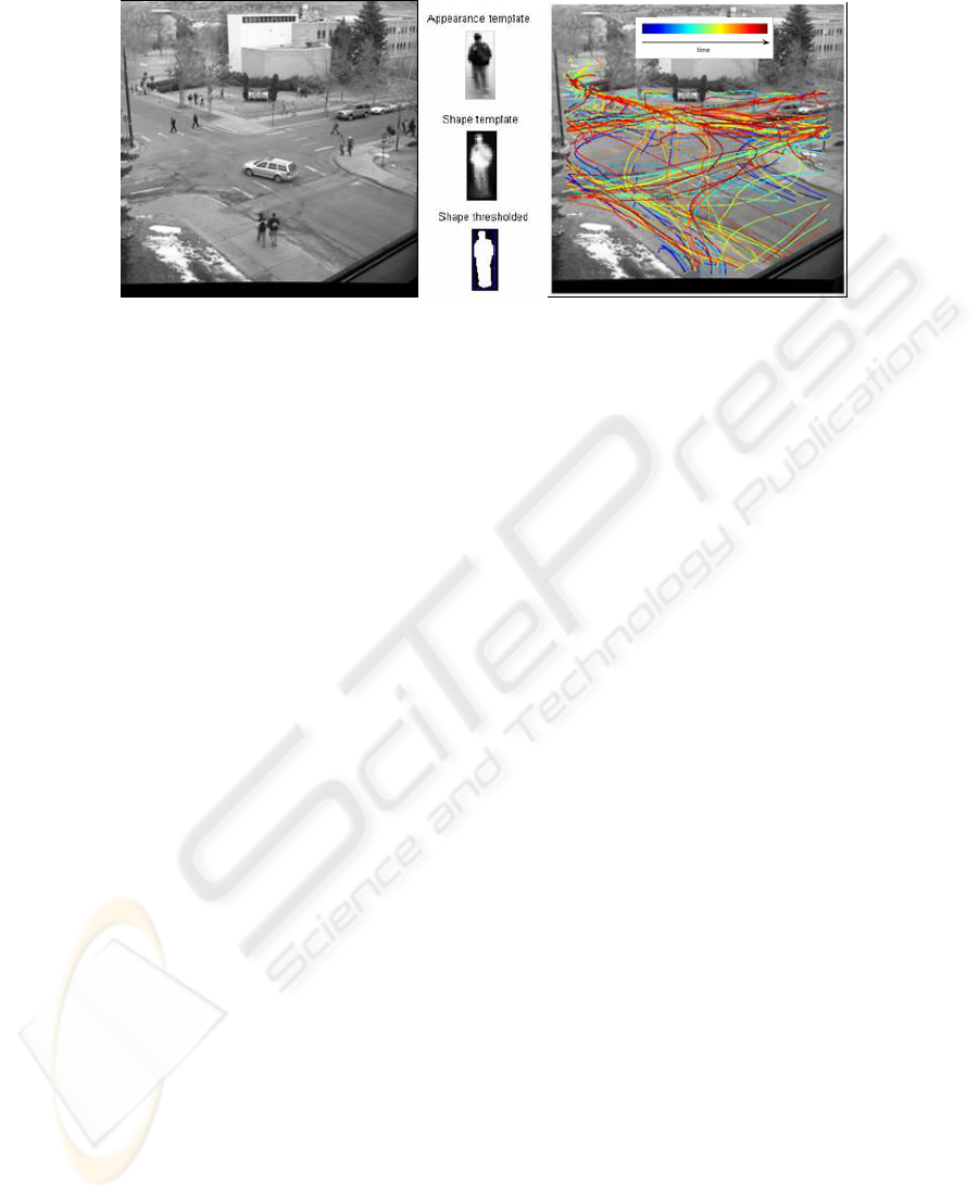
Fig. 1. Data collection and processing. (Left) Street intersection scene. (Center) The tracker
maintains templates of the shape and appearance of each object being tracked. (Right) Tracks
from street intersection scene
An automatic tracker program was developed to automatically track all moving ob-
jects in the scene and write their coordinates to a track file. First, a background, or
“reference” image was obtained by averaging all the images. Because moving ob-
jects tend to pass quickly in front of the background, they tend to average out.
The operation of the tracker was as follows:
1. Read in the next image of the sequence.
2. Take the difference between this image and the reference image. Threshold the
difference image and find connected components.
3. For each component that is not already being tracked from previous images, start a
new track. The track file information consists of the location of the object, its
“bounding box” in the image, and an “appearance template” of the object within
the bounding box. A “shape template” is also computed, which when thresholded
is a binary image of the silhouette of the object (Figure 1, center).
4. For each tracked object, perform a cross correlation operation to find the most
likely location of the template in the new image. Then update the template image
of the object by computing a running average of its image.
For the street scene, Figure 1 (right) shows all tracks obtained after 3 minutes. The
actual world coordinates were also computed, using the assumption of a flat world.
Very short tracks (less than 3 seconds) were discarded, because they were considered
to be due to noise. The (x,y) locations of the remaining tracks were smoothed by
running a low pass (Gaussian) filter, with σ = 0.4 seconds.
3 Visualization Tools
After tracks have been detected and measured, we perform the following steps:
1. Visualization/analysis of the results of motion tracking
2. Derivation of additional numerical attributes of motion tracks
3. Visualization of derived attributes
126
4. Classification of tracks and scenes
Data visualization is an important component of the process. Two visualization
tools, a track visualizer and an attribute visualizer, are described below. We used the
track visualizer to determine the accuracy of the track detection, which also provided
us with an improved understanding of the characteristics of the data that need to be
analyzed. This understanding led us to propose various numerical attributes of the
tracks that could be used to differentiate between different human activities. The
visualization of these attributes enabled us to formulate several different approaches
to classifying the tracks, and to validate or invalidate these approaches.
The track visualizer presents the motion tracks in a scene as a set of line segments
in the plane where they were detected (Figure 2, left). The motion can be animated
by translating symbols (e.g. colored cubes) along the tracks, illustrating the object’s
position over time. The video frames (from which the motion was detected) can be
replayed as an animated background. The user can match the detected motion tracks
with the moving objects in the video, and can spot discrepancies in the track
detection. The track visualization provides 3-D scene navigation, so that the user can
see the motion tracks from any direction. A background image of the scene is
displayed behind the tracks so that the user sees the tracks in the perspective of the
simulated physical position in the scene. The motion tracks and segments within the
tracks can be labeled, based on automatic or manual classification of the tracks.
Colors are applied to the tracks indicating the associated labels.
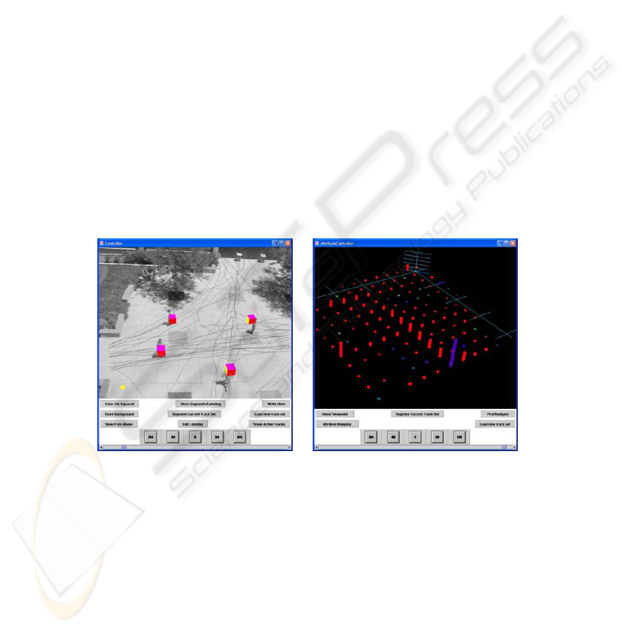
Fig. 2. Visualization tools. (Left) Motion tracks superimposed over the corresponding video
image. (Right) The attribute visualizer allows a general mapping of track attributes to scene
dimensions - this shows the distribution of starting(x,y) positions for actors in a scene
The attribute visualizer provides a 3-D animated display of numerical attributes as-
sociated with motion tracks or with segments within motion tracks. In this context,
an “attribute” is any (discrete or continuous) function that can be calculated from the
data associated with a motion track. Attributes to be plotted are specified as functions
of track segments, and can depend on any computed property of the track segment,
such as ground coordinates, speed, or orientation. The attributes can be defined by
127

Java routines (previously defined, then invoked at runtime) or calculated externally,
using, for example, MatLab™, to interactively calculate the values of the attribute
from the data associated with each track segment. The values of track attributes are
mapped at run time to any of a number of plotted dimensions, including x, y, and z
coordinates, time (i.e. animation frame number), color (hue, saturation and value),
transparency, symbol size, and symbol shape. The resulting animated graphs can be
compared to evaluate differences between numerical measures associated with the
scenes and with actors in the scenes. Histograms of track attributes are particularly
useful.
In Figure 2 (right) we show the visualization of some numerical properties of a
scene. The histogram indicates the frequency of starting x,y coordinates for tracks in
a scene. The histogram bars are color-coded according to the average turning angle
of the corresponding track segments.
4 Anomaly Detection
In this section, we describe our method for detecting anomalous activities based on
probability distributions. We can characterize scenes, and actors within these scenes,
by comparing the distributions of speed and turning angle for the actors in the scene.
The distributions are approximated by calculating histograms of these attributes.
Each actor is associated with a motion track, consisting of the actor’s position at
1/30th second intervals.
An average speed can be calculated between any pair of positions and times,
evaluated as distance divided by time. The turning angle is a number between -180
and 180 (degrees) determined from three successive positions on a motion track (and
the resulting direction angle change) separated by a specified time interval.
Given any scene, or a single actor within a scene, and for each time interval, there
is associated a histogram (approximating a probability distribution) describing the
distribution of speeds and turning angles in that scene, by one or all of the actors in
the scene. In the experiments we describe here, we chose a logarithmic sequence of
time scales, e.g. 1, 2, 4, 8, …, frames and calculated the histograms for each time
scale.
To compare actors or scenes, we used the chi-squared statistic as measure of the
similarity between two histograms. The chi-squared statistic is associated with two
binned variables, and can be used to compare the histograms associated with different
scenes, as well as the histograms associated with actors within these scenes [8]:
(
)
()
∑
+−=
i
iiii
SRSRSRSRSR
2
2
),(
χ
(1)
where
and
∑
=
i
i
RR
∑
=
i
i
SS .
The computed chi-square statistic is used to test the null hypothesis that two distri-
butions are the same. A relatively large value indicates that the two are not identical
(i.e., we reject the null hypothesis). We applied this statistic to distinguish one type
of sports scene from another, and the result is shown in Figure 3.
128
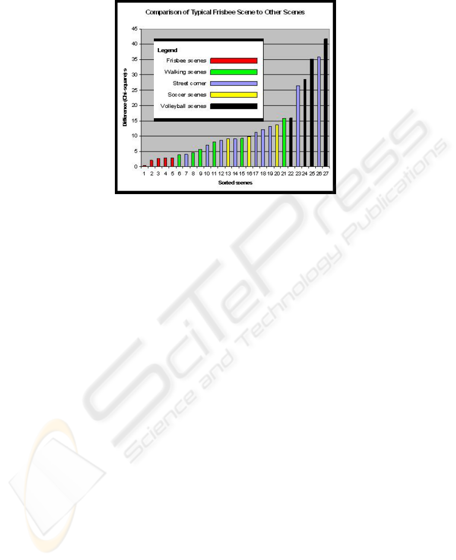
Fig. 3. A comparison of different scenes using the χ
2
-statistic, applied to the histograms of
turning angles and speeds. The plotted value is determined by applying equation (1) at each
scale, and then averaging these values of χ
2
Note the small values of χ
2
resulting from pairs of different “Ultimate Frisbee”
scenes, meaning that these scenes are similar to each other. On the other hand, the χ
2
value is larger when comparing the “Frisbee” scene to other unrelated activities such
as volleyball or walking through the street corner. This difference between histo-
grams is due to the fact that Frisbee players have typically much more high-speed and
high-turning intervals than actors in the other scenes.
Similarly, the χ
2
statistic was also applied to identify “unusual” activities within
scenes. Using equation (1), the histogram associated with each actor’s motion track
is compared with the histogram of all other actors in the scene (not including that
actor). In this case the method correctly identified the distributor of flyers as the most
“unusual” actor in the street scenes. This is likely due to the fact that the track for the
flyer distributor tends to meander, while the other actors tend to go straight through
the scene.
Thus, our method can detect unusual activities and scenes in an unsupervised man-
ner. The human supervisor can then inspect these unusual events and, if they are of
interest, label them. The system can then learn to recognize these activities using
machine learning methods, as is described in the next section.
5 Activity Classification
In this section, we describe our method for classifying activities using supervised
machine learning methods. Activity classifications can be proposed in an unsuper-
vised manner as discussed in the previous section, or provided directly by a human
user. The human-generated labels impose added complexity, as a person often resorts
to arbitrary boundaries between activity labels. The added complexity of human-
129

based class labels provides a more realistic example of our target application. We
examine two types of classification, namely motion-based and behaviour-based clas-
sifications. Motion-based classifications are strongly tied to attributes such as veloc-
ity or acceleration. Behaviour-based classifications are determined by a human user
from examining the context in which the activity occurs. These represent a much
more difficult set of classifications, as the feature set utilized does not take into ac-
count full contextual information.
We first divide tracks into equal length segments of approximately three seconds
in duration. (In a pilot study, we found through cross-validation that this segment
length provides a good balance between expressiveness of a segment and the number
of segments available for training.)
5.1 Feature Selection
We discarded absolute positional data because the position at which a behaviour
occurs is usually irrelevant in terms of describing the behaviour. Instead, we used
velocity, acceleration, speed, and turning rate computed at every position of a given
activity segment. Velocity and acceleration are vector quantities, and are computed at
each point of a track segment by use of the first and second forward difference, re-
spectively. The speed is the magnitude of its velocity, and the turning rate is the
difference in angle between the velocity vector at time t and t+1. Finally, we com-
pute the minimum, maximum, and average speed and turning rate over the activity
segment.
5.2 Motion Classifications
The first set of classifications we consider are motion based, meaning that the metric
is primarily based on overall speed of the segment. For the flyer scenes, an individual
distributes flyers to other individuals travelling through the area. The flyer person
meanders about the scene, occasionally intercepting others. The first motion classifi-
cation experiment matches a given activity segment to the label of “meandering” or
“normal” activity. A meander activity is loosely defined as any activity segment
where the individual is stopped completely, or is moving slowly in an indirect path.
To evaluate performance of machine learning classifiers, we perform ten times ten-
fold cross validation on a set of six classifiers. Two of these were “simple” classifiers
with high bias and low variance: (1) one-rule and (2) decision stumps. The others
were more “complex” classifiers: (3) decision tables (low bias, high variance), (4)
decision trees (low bias, high variance), (5) SVMs with Polynomial Kernel of power
2 (medium bias, medium variance), and (6) SVMs with Gaussian RBF Kernel of σ =
0.01 and regularization constant C=1000 (low bias, medium variance).
Model performance appears in Figure 5a. The majority of the models perform at
around 2% error. The SVM with RBF model has the best performance. All models
perform well on the activity segments except for the “one rule” model. This prelimi-
nary data set shows that our activity segmenting and modelling process performs
well.
130
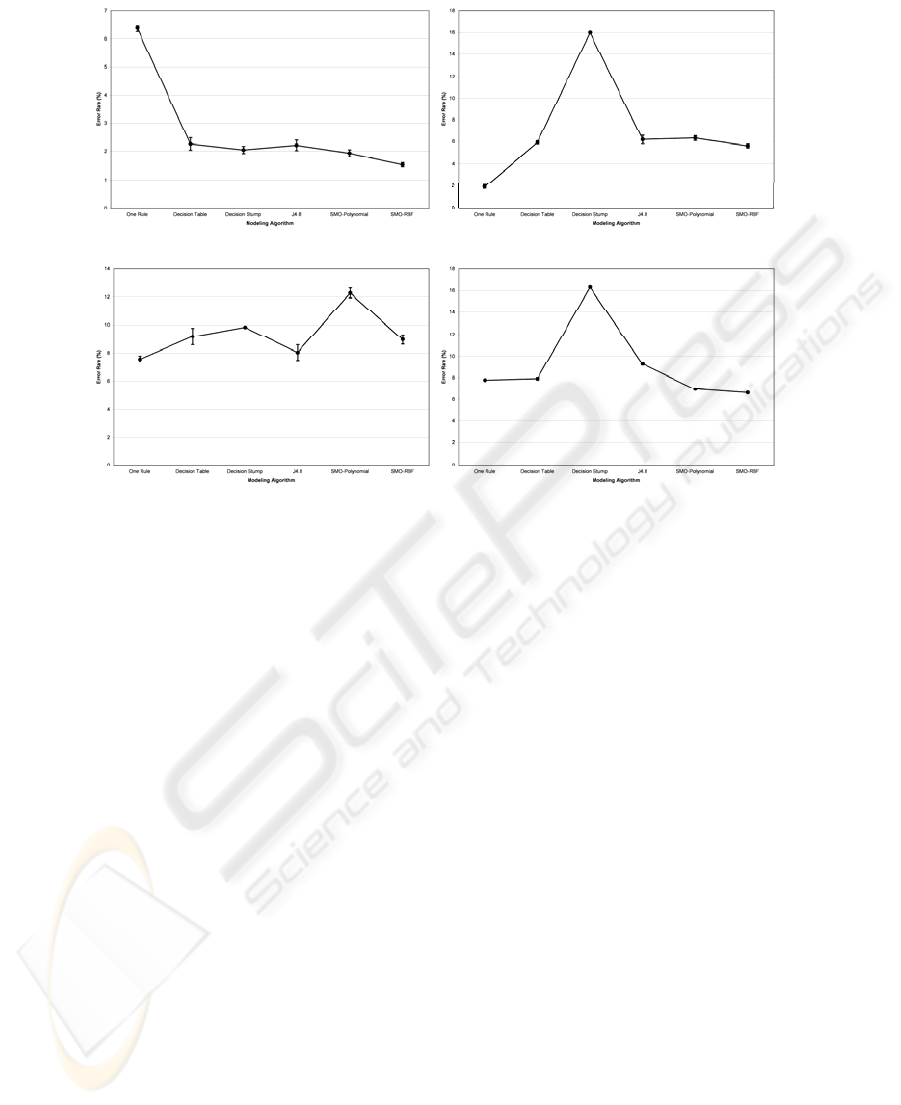
(a) (b)
(c) (d)
Fig. 4. (a) Performance on flyer scene, “meander” vs. “normal”. With the exception of the one
rule model, all of the modelling algorithms perform well on classifications based on motion.
(b) Flyer scene, multiple speed labels and cars. One rule outperforms all other classes with a
set of thresholds based on average speed. (c) Performance on sports scene, motion classifica-
tion (standing, walking, and running). (d) Performance on flyer scene, flyer behaviour vs.
other behaviours. Classification labels are assigned by the activity of the individuals in the
scene. One of the individuals in the scene is distributing flyers to others who pass through the
scene. As the nature of the flyer person’s behaviour is different, their motion track has differ-
ent properties
The second motion classification experiment is also based on the flyer scene. It
moves to a higher number of activities being distinguished. These are stopped, slow,
and normal-paced human motion, as well as all cars and bicycles grouped separately.
A speed-based threshold approach performs equally well here, as all that is necessary
is an additional threshold to differentiate slow activities from stopped activities. With
this experiment, we add in more of a behavioural classification in the car label, as
stopped and slow car activities are not extracted from the overall car motion track.
Model performance appears in Figure 5b. Most models perform around 6% error.
Decision stumps perform extremely poorly, due to its selection of a single attribute,
and a single threshold; it cannot represent more than two classes. One rule out per-
forms all others by far. As initial labelling of the activities was performed by a hu-
man user, the differences between what constitutes a slow activity versus a stopped or
normal-paced activity is not a hard threshold, though the threshold approach of one
rule performs well. As for the cars and bicycles, a concern was that their activity
signature would be too easily confused with a person, as the vehicles stop and move
131

slowly through the intersection. On the contrary, the majority of the cars and bicycles
are correctly classified. We attribute this in large part to the segment length selection,
where the greatest segment length possible is selected.
The third motion classification experiment switches to the sports scenes. Class la-
bels distinguish the basic motion pattern of a player between standing, walking, or
running. Added complexity arises due to the human-based class labels, as the divid-
ing thresholds between class labels is arbitrarily enforced by the person generating
the labels. There is likely a shift in class thresholds not only within sports, but across
sports as well. For example, a person who is labelled as walking in a soccer game
might be labelled as standing in a volleyball game, simply because of the context in
which the motion takes place. The added complexity of human-based class labels
provides a more realistic example of our target application.
Performance is reported in Figure 5c. As with the second motion experiment on
the flyer scene, decision stumps perform poorly due to the bias against decisions
involving more than two classes. Other than the decision stump model, the remaining
models perform between 6.6% and 9.3%. The best of these are the SVMs; the worst
is the decision tree. Performance is slightly poorer than with the second motion ex-
periment. The boundary between the activities was again allowed to be arbitrarily
defined by the human user performing the activity labelling. This may be part of the
impact on the performance.
For motion-based classifications, performance on all scenes is on average less than
10 % error rate. Our segmentation and feature selection process works well at model-
ling motion-based classifications.
5.3 Behavioural Classifications
Behaviours are much more difficult to express explicitly than motion-based classes,
as a single threshold cannot encapsulate all the variation which exists in a behaviour.
In generating a behavioural label, e.g., a Frisbee player or a flyer person, often an
entire motion track is placed in a behavioural class. This is not to preclude the possi-
bility of an individual exhibiting multiple behaviours over the duration of their mo-
tion track; rather, it is a result of the scenes which generate our motion data. We have
no occurrences of a travelling person stopping to distribute flyers, or of a soccer
player becoming a Frisbee player.
Our experiment classifies the flyer person versus all other individuals in the scene.
One might expect this problem to be very straightforward, as the behaviour of the
flyer person is distinct from other actors in the scene. On the other hand, there are
times when the flyer person exhibits behaviour which is similar to normal traffic, as
well as times when the travelling individuals stop or move slowly.
The flyer person has a signature which tends to meander about the scene, occa-
sionally moving to intercept others, and occasionally stopping to wait. Other indi-
viduals tend to travel at a constant pace through the scene, though at times they slow
or stop. Each track is labelled as either a normal behaviour or a flyer person behav-
iour. Modelling results are displayed in Figure 5d. The difference among modelling
algorithm performances is slightly more spread out. The range is from about 7.5% to
12.5% error. The best models are produced by one rule and decision tree. The worst
132

modelling algorithm at this task was the SVM constructed with the polynomial ker-
nel. In general, overall modelling performance is promising. The modelling tech-
niques were able to represent the ill-defined activities fairly well.
6 Conclusions
The results of the various experiments provide insight into the potential for
behavioral classification of motion tracks. In the motion-based classifications, a
simple metric was selected based loosely on the average speed of the individuals
being monitored. Specific thresholds separating the activities could have been used,
but the arbitrary assignment of categories by a human user requires more flexibility
from the modeling tools. These experiments stand as the preliminary proof of
concept that such classifications on motion tracks are attainable.
The behavioral classification experiment consists of an abstract label being
assigned with no regard for which of the available features might best help
distinguish between class labels. In the flyer scenes, the flyer person tended to move
in a different pattern than other travelers. This was sufficient to recognize the activity
in cross-validation experiments.
Preliminary work indicates that there is potential for improvement in modeling
behavioral data by the inclusion of windowing data. The improvement arises from an
extension of the information available where track length exceeds segment length.
The overall performance of our approach to motion and behavior classification is a
success.
References
1. A. Madabhushi and J. K. Aggarwal, "A Bayesian Approach to Human Activity Recogni-
tion," Proc. of Second IEEE Workshop on Visual Surveillance, Fort Collins, Colorado,
1999, Fort Collins, Colorado, June 26-26, pp. 25.
2. N. M. Oliver, B. Rosario, and A. P. Pentland, "A Bayesian computer vision system for
modeling human interactions," IEEE Trans. PAMI, vol. 22, no. 8, pp. 831-843, 2000.
3. M. Brand and V.Kettnaker, “Discovery and Segmentation of Activities in Video,” IEEE
Trans. PAMI, vol. 22, no. 8, pp. 844-851, 2000.
4. Y.A. Ivanov, and A. F. Bobick, “Recognition of Visual Activities and Interactions by Sto-
chastic Parsing,” IEEE Trans. PAMI, vol. 22, no. 8, pp. 852-871, 2000.
5. R. Nevatia, T. Zhao, and S. Hongeng, “Hierarchical language-based representation of events
in video stream,” CVPR Workshop ’03, 2003
6. I. Davidson, "Visualizing Clustering Results," Proc. of SIAM International Conference on
Data Mining, 2002.
7. N. Grady, R. J. Flanery, J. Donato, and J. Schryver, "Time Series Data Exploration," Proc.
of CODATA Euro-American Workshop, 1997, June.
8. W. H. Press, S. A. Teukolsky, W. T. Vetterling, and B. P. Flannery, Numerical Recipes in
C, 2nd ed: Cambridge University Press, 1992.
133
