
A Weighted Maximum Entropy Language Model for
Text Classification
Kostas Fragos
1
, Yannis Maistros
2
, Christos Skourlas
3
1 Department of Computer Engineering, National Technical University of Athens, Iroon
Polytexneiou 9 15780 Zografou Athens Greece
2 Department of Computer Engineering, National Technical University
of Athens, Iroon
Polytexneiou 9 15780 Zografou Athens Greece
3 Department of Computer Science, Technical Educational Institute of Athens, Ag Spy
ri-
donos 12210 Aigaleo Athens Greece
Abstract. The Maximum entropy (ME) approach has been extensively used in
various Natural Language Processing tasks, such as language modeling, part-
of-speech tagging, text classification and text segmentation. Previous work in
text classification was conducted using maximum entropy modeling with bi-
nary-valued features or counts of feature words. In this work, we present a
method for applying Maximum Entropy modeling for text classification in a
different way. Weights are used to select the features of the model and estimate
the contribution of each extracted feature in the classification task. Using the X
square test to assess the importance of each candidate feature we rank them and
the most prevalent features, the most highly ranked, are used as the features of
the model. Hence, instead of applying Maximum Entropy modeling in the clas-
sical way, we use the X square values to assign weights to the features of the
model. Our method was evaluated on Reuters-21578 dataset for test classifica-
tion tasks, giving promising results and comparably performing with some of
the “state of the art” classification schemes.
1 Introduction
Manual categorization of electronic digital documents is time-consuming and expen-
sive and its applicability is limited especially for very large document collections.
Consequently, text classification has increased in importance and economic value as
it is related to key technologies for classifying new electronic documents, extracting
interesting information on web and guiding users search through hypertext.
In early approaches to text classificat
ion a document representation model is em-
ployed based on term-based vectors. Such vectors are elements of some high dimen-
sional Euclidean space where each dimension corresponds to a term. Classification
algorithm and supervised learning training are usually applied.
Fragos K., Maistros Y. and Skourlas C. (2005).
A Weighted Maximum Entropy Language Model for Text Classification.
In Proceedings of the 2nd International Workshop on Natural Language Understanding and Cognitive Science, pages 55-67
DOI: 10.5220/0002571800550067
Copyright
c
SciTePress

A great number of text categorization and classifying techniques have been pro-
posed to the literature, including Bayesian techniques [1],[2],[3], k-Nearest Neighbors
(k-NN) classification methods [4],[5],[6], the Rocchio algorithm for Information
Retrieval [7],[8], Artificial Neural Networks (ANN) techniques [9],[10],[11],[12],
Support Vector Machines (SVM) learning method [13],[14],[15], Hidden Markov
Models (HMM) [19],[20], and Decision Tree (DT) classification methods
[17],[18],[9],[1]. In most of these methods, the aim is to estimate the parameters of
the joint distribution between the object X, that we want to be classified, and a class
category C and assign the object X to the category with the greater probability. Un-
fortunately, the complexity of the problem in real-world applications implies that the
estimation of the joint distribution is a difficult task. In general such an estimation
involves a potentially infinite set of calculations over all possible combinations of X
and elements of C. Using the Bayes formula the problem can be decomposed to the
estimation of two components P(X|C) and P(C), known as the conditional class dis-
tribution and prior distribution, respectively.
Maximum Entropy (ME) modeling could be seen as an intuitive way for estimating
a probability and has been successfully applied in various Natural Language Process-
ing (NLP) tasks such as language modeling, part-of-speech tagging and text segmen-
tation [23],[24],[25],[26],[28],[29]. The main principle underlying ME is that the
estimated conditional probability should be as uniform as possible (have the “maxi-
mum entropy”). The main advantage of ME modeling for the classification task is
that it offers a framework for specifying any potentially relevant information. Such
information could be expressed in the form of feature functions, the mathematical
expectations (constraints) of which are estimated based on labeled training data and
characterize the class-specific expectations for the distribution. The main principle of
ME could also be seen in the following way: “Among all the allowed probability
distributions, which conform to the constraints of the training data, the one with the
maximum entropy (the most uniform) is chosen”. It can be proved that there is a
unique solution for this problem. The uniformity of the solution found, a condition
known as the “lack of smoothing”, may be undesirable in some cases. For example, if
we have a feature that always predicts a certain class then this feature can be assigned
to a high ranked weight. Another potential shortcoming of the ME modeling is that
the algorithm which is used to find the solution can be computationally expensive due
to the complexity of the problem.
In this work, we try to eliminate the above undesirable situations. As it is well
known, X square statistic has been widely used in NLP tasks. The X square test for
independence can be applied to problems where data is divided into mutual exclusive
categories and has the advantage that it does not assume normally distributed prob-
abilities. The “essence” of the test is to assess the assumption that is related to the
independence of an object X from a category. If the difference between the observed
and expected frequency is great we can reject the assumption about the independence
(null hypothesis). Every word term w in a document d is seen as a candidate feature
and the X square statistic is used to test the independence of the word w (with each
element of the Class Categories c). This test is conducted by counting the (observed)
frequencies of the word, in each class category of the training set. Then the resulting
value of the test is used to select the most representative features for the maximum
56

entropy model as well as to assign weights to the features giving different importance
for the classification task in each one of them.
In section 2 the application of the X square test for feature extraction based on a
sample of data and the related weighting scheme are discussed. In section 3 the maxi-
mum entropy modeling and the improved iterative scaling (IIS) algorithm are pre-
sented. In section 4 we discuss the way of using maximum entropy modeling for text
classification. In section 5 the experimental results are presented and briefly discussed
and in section 6 the conclusions and future activities are given.
2 X Square Test for Feature Selection
Among the most challenging tasks in the classification process, we can distinguish
the selection of suitable features to represent the instances of a particular class. Addi-
tionally, the choice of the best candidate features can be a real disadvantage for the
selection algorithm, in terms of effort and time consumption [22].
As it has been mentioned above, each document is represented as a vector of
words, as is typically done in the Information Retrieval approach. Although in most
text retrieval applications the entries (constituents) of a vector are weighted to “re-
flect” the importance of the term, in text classification simpler binary feature values
(i.e., a term either occurs or does not occur in a document) are often used. Usually,
text collections contain millions of unique terms and for reasons of computational
efficiency and efficacy, feature selection is an essential step when applying machine
learning methods for text categorization. In this work, the X square test is used to
reduce the dimensionality of data and is also related to the maximum entropy model-
ing.
In 1900, Karl Pearson developed a statistic that compares all the observed and ex-
pected values (numbers) when the possible outcomes are divided into mutually exclu-
sive categories. The chi-square statistic is expressed by the following equation 1:
(1)
Where Greek letter Σ stands for the summation and is calculated over the catego-
ries of all possible outcomes.
The observed and expected values can be explained in the context of hypothesis
testing. If data is divided into mutual exclusive categories and we can form a null
hypothesis about the sample of the data, then the expected value is the value of each
category if the null hypothesis is true. The observed value for each category is the
value that we observe from the sample data.
The chi-square test is a reliable way of gauging the significance of how closely the
data agree with the detailed implications of a null hypothesis.
To clarify things let us see an example based on data from Reuters-21578. Suppose
that we have two distinct class categories c
1
= ’Acq’ and c
2
≠ ’Acq’ extracted from
the Reuters-21578 ‘ModApte’ split training data set. We are interested in assessing
the independence of the word ‘usa’ from the elements of class categories c
1
and c
2
.
57

From the training data set we remove all the numbers and the words that exist in the
stopword list. Counting the frequencies of the word ‘usa’ in the training dataset we
find that the word ‘usa’ appears in the class Acq (c1=’Acq’) 1,238 times, and in the
other categories (classes), which means that the word is in the class (c
2
≠ ’Acq’),
4,464 times. In the class ‘Acq’ there is a total of 125,907 word terms while in the
other classes a total of 664,241. A total of N=790,148 word terms is contained in the
Reuters-21578 training dataset. It would be useful to use the contingency table 1 in
which the data are classified.
Table 1. Contigency table of frequencies for the word usa and the class Acq (calculation based
on Reuters-21578 ‘ModApte’ split training dataset)
c
1
= ‘Acq’ c
2
≠ ’Acq’
Total
w =
‘usa’ 1,238 4,464
5,702
w ≠ ‘usa’
124,669 659,777
784,446
Total
125,907 664,241
N=
790,148
The assumption about the independence (null hypothesis) is that occurrences of the
word ‘usa’ and the class label ‘Acq’ are independent.
We compute now the expected number of observations (frequencies) in each cell
of the table if the null hypothesis is true. These frequencies can be easily determined
by multiplying the appropriate row and column totals and then dividing by the total
number of observations.
Expected frequencies:
w= ’usa’ and c1=’Acq’: E
11
= (5,702x125,907)/790,148 = 908.59
w= ’usa’ and c1≠’Acq’: E
12
= (5,702x664,241)/790,148 = 4,793.4
w≠ ’usa’ and c1=’Acq’: E
21
= (784,446x125,907)/790,148 = 124,998.4
w≠ ’usa’ and c1≠’Acq’: E
22
= (784,446x664,241)/790,148 = 659,447.6
Using equation 1 we calculate the X
2
value:
X
2
=(1,238-908.59)
2
/908.59 + (4,464-4793.4)
2
/4793.4 +
(124,669-124,998.4)
2
/124,998.4 + (659,777-659,447.6)
2
/659,447.6
= 143.096.
Then we calculate the X
2
value using eq. 1. We find a critical value for a signifi-
cance level a (usually a=0.05) and for one degree of freedom (the statistic has one
degree of freedom for a 2x2 contingency table). If the calculated value is greater than
the critical value we can reject the null hypothesis that the word ‘usa’ and the class
label ‘Acq’ occur independently. So, for a calculated great X
2
value we have a strong
evidence for the pair (‘usa’, ‘Acq’). Hence, the word ‘usa’ is a good feature for the
classification in the category ‘Acq’.
To make things simpler, we are only interested in calculating great X
2
values. Our
aim is to choose the most representative features among the large number of candi-
dates and perform classification in a lower dimensionality space.
For a contingency 2-by-2 table the X square values can be calculated by the fol-
lowing formula 2:
(2)
58

Where a
ij
are the entries of the contingency 2-by-2 table A and N the total sum of
these entries.
Chi-square test has been used in the past for feature selection in text classification
field. Yang and Pedersen [34] compared five measurements in term selection, and
found that the chi-square and information gain gave the best performance.
3 Maximum Entropy Approach
3.1 Maximum Entropy Modeling
The origin of Entropy can be traced in the dates of Shannon [27] when this concept
was used to estimate how much data could be compressed before the transmission
over a communication channel. The entropy H measures the average uncertainty of a
single random variable X:
)(log)()()(
2
xpxpXHpH
Xx
∑
∈
−==
(3)
Where, p(x) is the probability mass function of the random variable X. Equation 4
also calculates the average number of bits we need to transfer all the information.
Formula 3 is used in the communication theory to save the bandwidth of a communi-
cation channel. We prefer a model of X with less entropy so that we can use smaller
bits to interpret the uncertainty (information) inside X. However in NLP tasks we
want to find a model to maximize the entropy. This sounds as though we are violating
the basic principle of entropy. Actually, we try to avoid “bias” when the certainty
cannot be identified from the empirical evidence.
Many problems in NLP could be re-formulated as statistical classification prob-
lems. Text classification task could be seen as a random process Y which takes as
input a document d and produces as output a class label c. The output of the random
Y may be affected by some contextual information X. The domain of X contains all
the possible textual information existing in the document d. Our aim is to specify a
model p(y|x) which denotes the probability that the model assigns y
∈
Y when the
contextual information is x
∈
X. The notation of this section follows that of Adam
Berger [28] [29] [35].
On the first step, we observe the behavior of the random process in a training sam-
ple set collecting a large number of samples (x
1
, y
1
), (x
2
, y
2
)…(x
N
, y
N
). We can sum-
marize the training sample defining a joint empirical distribution over x and y from
these samples:
samplethein) occurstimes (x,ynumber of
N
yxp ×=
1
),(
~
(4)
One way to represent contextual evidence is to encode useful facts as features and
to impose constraints on values of those feature expectations. This is done in the
following way. We introduce the indicator function [28] [35]
59

{
'2_''1_'1
0
),(
valuesomexandvaluesomeyif
otherwise
yxf
=
=
=
(5)
For example, in our classification problem an indicator function may be f(x,y)=1 if
y=’c
1
’ and x contains the word ‘money’ and f(x,y)=0 otherwise. Where ‘c
1
’ is a par-
ticular value from the class labels and x is the context (the document) where the word
‘crude’ occurs within. Such an indicator function f is called a feature function or
feature for short. Its mathematical expectation with respect to the model p(y|x) is
),(),(
,
~
yxfyxp
yx
∑
(6)
We can ensure the importance of this statistic by specifying that the expected value
that the model assigns to the corresponding feature function is in accordance with the
empirical expectation of equation 7.
),(),(),()|()(
,,
~~
yxfyxpyxfxypxp
yxyx
∑∑
=
(7)
where
is the empirical distribution of x in the training sample. )(
~
xp
We call the requirement equation 7 a constraint equation or simply a constraint
[28][35].
When constraints are estimated, there are various conditional probability models
which can be applied and satisfy these constraints. Among all these models there is
always a unique distribution that has the maximum entropy and it can be shown [30]
that the distribution has an exponential form:
⎟
⎠
⎞
⎜
⎝
⎛
=
∑
i
ii
yxf
xZ
xyp ),(exp
)(
1
)|(
λ
λ
λ
(8)
where Z(x) a normalizing factor to ensure a probability distribution given by
∑∑
⎟
⎠
⎞
⎜
⎝
⎛
=
yi
ii
yxfxZ ),(exp)(
λ
λ
(9)
where λ
i
a parameter to be estimated, associated with the constraint f
i
.
The solution, which is related to the maximum entropy model and is calculated by
the equation 9, is also the solution to a dual maximum likelihood problem for models
of the same exponential form. It means that the likelihood surface is convex, having a
single global maximum and no local maximum. There is an algorithm that finds the
solution performing Hill Climbing in likelihood space.
60

3.2 Improved Iterative Scaling
We describe now a basic outline of the improved iterative scaling (IIS) algorithm, a
Hill Climbing algorithm for estimating the parameters λ
i
of the maximum entropy
model, specially adjusted for text classification. The notation of this section follows
that of Nigam et al. [31] with x to represent a document d and y a class label c.
Given a set of training dataset D, which consists of pairs (d, c(d)), where d the docu-
ment and c(d) the class label in which the document belongs, we can calculate the
loglikelihood of the model of equation 9.
),(explog
)(,()|)((log)|(
cdf
dcdfddcpDpL
i
Ddci
i
Dd
i
i
i
Dd
∑∑∑
∑
∑
∏
∈
∈
∈
−==
λ
λ
λλ
(10)
The algorithm is applicable whenever the feature functions f
i
(d,c(d)) are non-
negative.
To find the global maximum of the likelihood surface, the algorithm must start
from an initial exponential distribution of the correct form (that is to “guess” a start-
ing point) and then perform Hill Climbing in likelihood space. So, we start from an
initial value for the parameters λ
i
, say λ
i
=0 for i=1:K (where K the total number of
features) and in each step we improve by setting them equal to λ
i
+δi, where δi is the
increment quantity. It can be shown that at each step we can find the best δi by solv-
ing the equation:
∑
∑
∈
=
Ddc
ii
cdfdcpdcdf )),(exp()|())(,((
#
δ
λ
(11)
Where f
#
(d,c) is the sum of all the features in the training instance d.
Equation 12 can be solved in a “closed” form if the f
#
(d,c) is constant, say M, for
all d, c [28][31].
∑
∑
∈
=
c
i
Dd
i
i
dcfdcp
dcdf
M ),()|(
))(,(
log
1
λ
δ
(12)
where p
λ
(c|d) is the distribution of the exponential model of equation 9.
If this is not true, then equation 12 can be solved using a numeric root-finding pro-
cedure, such as Newton’s method.
However in this case, we can still solve equation 12 in “closed” form by adding an
extra feature to provide that f
#
(d,c) will be constant for all d, c, in the following way:
We define M as the greatest possible feature sum:
∑
=
=
K
i
i
cd
cdfM
1
,
),(max
(13)
61

and add an extra feature, that is defined as follows:
∑
=
+
−=
K
i
iK
cdfMcdf
1
1
),(),(
(14)
Now we can present an improved iterative scaling algorithm (IIS)
Begin
Add an extra feature f
K+1
following equations 13,14
Initialize •
i
=0 for i=1:K+1
Repeat
Calculate the expected class labels p
•
(c|d)
for each document with the current parameters
using equation 9
calculate •
i
from equation 12
set •
i
= •
i
+ •
i
Until convergence
Output: Optimal parameters •
i
optimal model p
•
End
4 Maximum Entropy Modeling for Text Classification
The basic shortcoming of the IIS algorithm is that it may be computationally expen-
sive due to the complexity of the classification problem. Moreover, the uniformity of
the found solution (lack of smoothing) can also cause problems. For example, if we
have a feature that always predicts a certain class, then this feature may be assigned to
an excessively high weight. The innovative point in this work is to use the X square
test to rank all the candidate feature words, that is, all the word terms that appear in
the training set and then select the most highly ranked of them for use in the maxi-
mum entropy model.
If we decide to select the K most highly ranked word terms w
1
, w
2
, …, w
K
we instan-
tiate the features as follows:
⎪
⎩
⎪
⎨
⎧
=
settrainingtheinappears
cdpairanddinoccurs
i
wwordifixsquare
otherwise
cdf
i
),()(
0
),(
(15)
where xsquare(i) denotes the X square score of the word w
i
obtained during the
feature selection phase.
This way of instantiating features has two advantages: first it gives a weight to each
feature and second it creates a separate list of features for each class label. The fea-
tures from each list can be different from class to class. These features are activated
only with the presence of the particular class label and are strong indicators of it. Of
course some features are common to more than one classes. These lists of features are
used from the resulting binary text classifier (the optimal model of the IIS algorithm)
62

to calculate the expected class labels probabilities for a document d, equation 9, and
then to assign the document d to the class with the highest probability.
5 Experimental Results
We evaluated our method using the “ModApte” split of the Reuters-21578 dataset
compiled by David Lewis. The “ModApte” split leads to a corpus of 9,603 training
documents and 3,299 test documents. We choose to evaluate only ten (10) categories
(from the 135 potential topic categories) for which there is enough number of training
and test document examples. We want to built a binary classifier and we split the
documents into 2 groups: ‘Yes’ group, the document belongs to the category and
‘No’ group, the document does not belong to the category. The 10 categories with the
number of documents for the training and test phase are shown in table 2.
Table 2. 10 categories from the “ModApte” split of the Reuters-21578 dataset and the number
of documents for the Training and the Test phase for a binary classifier.
Train Test
Category
Yes No Yes No
Acq 1615 7988 719 2580
Corn 175 9428 56 3243
Crude 383 9220 189 3110
Earn 2817 6786 1087 2212
Grain 422 9181 149 3150
Interest 343 9260 131 3168
Money-
fx
518 9085 179 3120
Ship 187 9416 89 3210
Trade 356 9247 117 3182
Wheat 206 9397 71 3228
In the training phase 9,603 documents were parsed. We avoid stemming of the
words and simply removed all the numbers and the words contained in a stopword
list. This preprocessing phase calculated 32,412 discrete terms of a total of 790,148
word terms. The same preprocessing phase was conducted in the test phase.
We applied the X square test to the corpus of those features (see section 3) and
then we selected for the maximum entropy model the 2,000 most highly ranked word
terms for each category. Table 3 presents for each category the 10 top ranked word
terms calculated by the X square test.
63

Table 3. 10 top ranked words calculated by the X square test for the 10 categories (the
ModApte Reuters-21578 training dataset)
Acq Corn Crude Earn Grain
bgas
annou
ameritech
calny
adebayo
echoes
affandi
f8846
faded
faultered
values
july
egypt
agreed
shipment
belgium
oilseeds
finding
february
permitted
Crude
Comment
Spoke
stabilizing
cancel
shipowners
foresee
sites
techniques
stayed
earn
usa
convertible
moody
produce
former
borrowings
caesars
widespread
honduras
Filing
Prevailing
Outlined
Brian
Marginal
Winds
Proceedings
neutral
requiring
bangladesh
Interest Money-fx Ship Trade Wheat
money
fx
discontin-
ued
africa
signals
anz
exploration
program
tuesday
counterparty
flexible
conn
proposals
soon
requirement
slow
soybeans
robert
calculating
speculators
acq
deficit
buy
officials
price
attempt
mitsubishi
mths
troubled
departments
trade
brazil
agreement
chirac
communications
growth
restraint
ran
slowly
conclusion
rumors
monetary
eastern
policy
cbt
storage
proposal
reuter
usually
moisture
Table 4. Micro-average Breakeven performance for 5 different learning algorithms explored
by Dumais et al. Comparison with WMEM algorithm
FindSim NBaye
s
Bayes-
Nets
Trees LinearSVM WMEM
Earn
92.9% 95.9% 95.8% 97.8% 98.2% 97.98%
acq
64.7% 87.8% 88.3% 89.7% 92.7% 87.93%
money-
fx
46.7% 56.6% 58.8% 66.2% 73.9% 75.09%
grain
67.5% 78.8% 81.4% 85.0% 94.2% 83.37%
crude
70.1% 79.5% 79.6% 85.0% 88.3% 72.20%
trade
65.1% 63.9% 69.0% 72.5% 73.5% 48.16%
interest
63.4% 64.9% 71.3% 67.1% 75.8% 64.21%
ship
49.2% 85.4% 84.4% 74.2% 78.0% 50.22%
wheat
68.9% 69.7% 82.7% 92.5% 89.7% 69.88%
corn
48.2% 65.3% 76.4% 91.8% 91.1% 57.36%
Using the 2000 most highly ranked word terms for each category we instantiate the
features of the maximum entropy model (see section 4). Using a number of 200 itera-
tions in the training phase of classifier, the IIS algorithms outputs the optimal λ
i
’s,
64
that is the optimal model p
λ
(c|d). We call this method Weighted Maximum Entropy
Modeling (WMEM) to emphasize the event that we use selected features and assign
weights to them.
To evaluate the classification performance of the binary classifiers we use the so-
called precision/recall breakeven point, which is the standard measure of perform-
ance in text classification and is defined as the value for which precision and recall
are equal. Precision is the proportion of items placed in the category that really be-
long to the category, and Recall is the proportion of items in the category that are
actually placed in the category. Table 4 summarizes the breakeven point performance
for 5 different learning algorithms based on research conducted by Dumais et al. [32]
and for our Weighted Maximum Entropy Model over the 10 most frequent Reuters
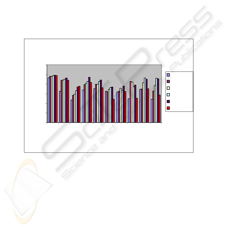
categories. Figure 1 is a graphical representation of the system’s performances to help
to compare the approaches more easily.
Breakeven point performance for 5 different learning algorithms
and for WMEM algorithm
0
20
40
60
80
100
120
e
ar
n
acq
m
oney-fx
grai
n
cr
u
de
trad
e
in
te
rest
ship
wh
e
at
co
rn
Categories
Performance
Findsim
Nbayes
BayesNets
Trees
LinearSVM
WMEM
Fig. 1. Breakeven performance calculated over the top ten (10) categories of the Reuters-21578
dataset. The Weighted Maximum Entropy Model (WMEM is the last one) is compared to five
(5) learning algorithms explored by Dumais et al.
Calculations illustrated in the Table 4 and Fig. 1 show that our method gives prom-
ising results especially in the case of the larger categories. It performs better than the
other classifiers in the ‘money-fx’ category and outperforms most of the other classi-
fiers in some of the largest in test size categories like ‘earn’, ‘acq’ and ‘grain’.
65

6 Discussion and Future Work
There are three other works using maximum entropy for text classification: The work
of Ratnaparkhi [26] is a preliminary experiment that uses binary features. The work
of Mikheev [33] examines the performance of the maximum entropy modeling and
conducts feature selection for text classification on the RAPRA corpus, a corpus of
technical abstracts. In this work binary features were also used. Nigam et al. [31] use
counts of occurrences instead of binary features and they show that maximum en-
tropy is competitive to and sometimes better than naïve Bayes classifier.
In this work, we have extended the previous research results using a feature selection
strategy and assigning weights to the features calculated by the X square test. The
results of the evaluation are very promising. However, the experiments will be con-
tinued in two directions. We shall conduct new experiments changing the number of
the selected features and / or the selection strategy, as well as the number of the itera-
tions in the training phase. Additional experiments using alternative datasets such as,
the WebKB dataset, the Newsgroups dataset etc., will be conducted in order to accu-
rately estimate the performance of the proposed method.
Acknowledgements
This work was co-funded by 75% from the E.U. and 25% from the Greek Govern-
ment under the framework of the Education and Initial Vocational Training Program
– Archimedes.
References
1. Lewis, D. and Ringuette, M., A comparison of two learning algorithms for text categoriza-
tion. In The Third Annual Symposium on Document Analysis and Information Retrieval
pp.81-93, 1994
2. Makoto, I. and Takenobu, T., Cluster-based text categorization: a comparison of category
search strategies, In ACM SIGIR'95, pp.273-280, 1995
3. McCallum, A. and Nigam, K., A comparison of event models for naïve Bayes text classifi-
cation, In AAAI-98 Workshop on Learning for Text Categorization, pp.41-48, 1998
4. Masand, B., Lino, G. and Waltz, D., Classifying news stories using memory based reason-
ing, In ACM SIGIR'92, pp.59-65, 1992
5. Yang, Y. and Liu, X., A re-examination of text categorization methods, In ACM SIGIR’99,
pp.42-49, 1999
6. Yang, Y., Expert network: Effective and efficient learning from human decisions in text
categorization and retrieval, In ACM SIGIR'94, pp.13-22, 1994
7. Buckley, C., Salton, G. and Allan, J., The effect of adding relevance information in a rele-
vance feedback environment, In ACM SIGIR’94, pp.292-300, 1994
8. Joachims, T., A probabilistic analysis of the rocchio algorithm with TFIDF for text catego-
rization, In ICML’97, pp.143-151, 1997
9. Guo, H. and Gelfand S. B., Classification trees with neural network feature extraction, In
IEEE Trans. on Neural Networks, Vol. 3, No. 6, pp.923-933, Nov., 1992
66

10. Liu, J. M. and Chua, T. S., Building semantic perception net for topic spotting, In ACL’01,
pp.370-377, 2001
11. Ruiz, M. E. and Srinivasan, P., Hierarchical neural networks for text categorization, In
ACM SIGIR’99, pp.81-82, 1999
12. Schutze, H., Hull, D. A. and Pedersen, J. O., A comparison of classifier and document
representations for the routing problem, In ACM SIGIR’95, pp.229-237, 1995
13. Cortes, C. and Vapnik, V., Support vector networks, In Machine Learning, Vol.20, pp.273-
297, 1995
14. Joachims, T., Learning to classify text using Support Vector Machines, Kluwer Academic
Publishers, 2002
15. Joachims, T., Text categorization with Support Vector Machines: learning with many
relevant features, In ECML’98, pp.137-142, 1998
16. Schapire, R. and Singer, Y., BoosTexter: A boosting-based system for text categorization,
In Machine Learning, Vol.39, No.2-3, pp.135-168, 2000
17. Breiman, L., Friedman, J. H., Olshen, R. A., and Stone, C.J., Classification and Regression
Trees, Wadsworth Int. 1984
18. Brodley, C. E. and Utgoff, P. E., Multivariate decision trees, In Machine Learning, Vol.19,
No.1, pp.45-77, 1995
19. Denoyer, L., Zaragoza, H. and Gallinari, P., HMM-based passage models for document
classification and ranking, In ECIR’01, 2001
20. Miller, D. R. H., Leek, T. and Schwartz, R. M., A Hidden Markov model information
retrieval system, In ACM SIGIR’99, pp.214-221, 1999
21. Kira, K. and Rendell, L. A practical approach to feature selection. In Proc. 9
th
International
workshop on machine learning (pp. 249-256) 1992
22. Gilad-Bachrach, Navot A., Tishby N. Margin Based Feature Selection - Theory
and Algorithms. In Proc of ICML 2004
23. Stanley F. Chen and Rosenfeld R. A Gaussian prior for smoothing maximum entropy mod-
els. Technical report CMU-CS-99108, Carnegie Mellon University, 1999
24. Ronald Rosenfeld. Adaptive statistical language modelling: A maximum entropy approach,
PhD thesis, Carnegie Mellon University, 1994
25. Ratnparkhi Adwait, J. Reynar, S. Roukos. A maximum entropy model for prepositional
phrase attachment. In proceedings of the ARPA Human Language Technology Workshop,
pages 250-255, 1994
26. Ratnparkhi Adwait. A maximum entropy model for part-of-speech tagging. In Proceedings
of the Empirical Methods in Natural Language Conference, 1996
27. Shannon C.E. 1948. A mathematical theory of communication. Bell System Technical
Journal 27:379 – 423, 623 – 656
28. Berger A, A Brief Maxent Tutorial. http://www-2.cs.cmu.edu/~aberger/maxent.html
29.Berger A. 1997. The improved iterative scaling algorithm: a gentle introduction
http://www-2.cs.cmu.edu/~aberger/maxent.html
30. Della Pietra S., Della Pietra V. and Lafferty J., Inducing features of random fields. IEEE
transaction on Pattern Analysis and Machine Intelligence, 19(4), 1997
31. Nigam K., J. Lafferty, A. McCallum. Using maximum entropy for text classification, 1999
32. Dumais, S. T., Platt, J., Heckerman, D., and Sahami, M, Inductive learning algorithms and
representations for text categorization. Submitted for publication, 1998
http://research.microsoft.com/~sdumais/cikm98.doc
33. Mikheev A., Feature Lattics and maximum entropy models. In machine Learning,
McGraw-Hill, New York, 1999
34. Yang, Y. and Pedersen J., A comparative study on feature selection in text categorization.
Fourteenth International Conference on Machine Learning (ICML’97) pp 412-420, 1997
35. Berger A., Della Pietra S., Della Pietra V., A maximum entropy approach to natural
language processing, Computational Linguistics, 22 (1), pp 39-71, 1996
67
