
Novel Circular-Shift Invariant Clustering
Dimitrios Charalampidis
University of New Orleans, Electrical Engineering Department, 2000 Lakeshore Dr.
New Orleans, Louisiana, 70148, United States
Abstract. Several important pattern recognition applications are based on feature
extraction and vector clustering. Directional patterns may be represented by rota-
tion-variant directional vectors, formed from M features uniformly extracted in M
directions. It is often required that pattern recognition algorithms are invariant under
pattern rotation or, equivalently, invariant under circular shifts of such directional
vectors. This paper introduces a K-means based algorithm (Circular K-means) to
cluster vectors in a circular-shift invariant manner. Thus, the algorithm is appropri-
ate for rotation invariant pattern recognition applications. An efficient Fourier do-
main implementation of the proposed technique is presented to reduce computa-
tional complexity. An index-based approach is proposed to estimate the correct
number of clusters in the dataset. Experiments illustrate the superiority of CK-
means for clustering directional vectors, compared to the alternative approach that
uses the original K-means and rotation-invariant vectors transformed from rotation-
variant ones.
1 Introduction
Texture analysis and object recognition have attracted great interest due to their large
number of applications, including medicine, remote sensing [13], and industry. The term
object may either be used to describe high level structures such as a vehicles or build-
ings, or low level image components such as edges or junctions. Both texture analysis
and object recognition may require that the image be segmented into several regions. In
general, the first step in the segmentation process is feature extraction. More specifi-
cally, multiple features are extracted from different image regions to form vectors repre-
senting those regions. Vector clustering [1]-[7] is usually the second step in the process.
Similar vectors may correspond to similar regions, therefore clustering results in a seg-
mented image. Generally, it is desirable that the segmentation process is invariant under
image rotations, rotation invariant features may be needed. Such invariance is usually
achieved by transforming rotation variant vectors into rotation invariant vectors. In this
approach, M features, {f
m
, m = 0, 1,…, M – 1}, may be uniformly extracted from M
directions defined by the angle
θ
m
= 360
o
m/M to form a rotational variant M-
dimensional vector F
d
= [f
0
, …, f
M-1
]. Traditionally, this feature vector may be trans-
formed into a rotational invariant vector [8]-[11]. The problem with transforming rota-
tion variant to rotation invariant feature vectors is that such a transformation results in
Charalampidis D. (2005).
Novel Circular-Shift Invariant Clustering.
In Proceedings of the 5th International Workshop on Pattern Recognition in Information Systems, pages 33-42
DOI: 10.5220/0002568500330042
Copyright
c
SciTePress

some loss of information. For instance, consider the Discrete Fourier Transform
(DFT) coefficient magnitudes |DFT{F
d
}| of vector F
d
defined above. These coeffi-
cients are invariant under image rotation by increments of 360
o
/M, since such a rota-
tion causes a circular shift of vector F
d
. Some preprocessing [8] may achieve invari-
ance of the DFT magnitude coefficients under any rotation. However, useful DFT
phase information is ignored.
An impractical solution to the problem of information loss would be to examine
all possible circular shifts for all vectors, and determine the best vector-grouping case
regardless of the shift. On the other hand, rotation invariance can be effectively
achieved by clustering the original feature vectors F
d
using a circular-shift invariant
clustering algorithm that causes no information loss. This paper introduces an algo-
rithm, namely Circular K-means (CK-means), for clustering vectors with directional
information, such as vector F
d
in a circular invariant manner. Furthermore, an efficient
Fourier domain representation of CK-means is presented to reduce computational
complexity. An index based approach is proposed for estimating the correct number
of clusters (CNC). The performance of CK-means has been tested on textural images.
The paper is organized as follows: In Section 2, the CK-means clustering algo-
rithm is introduced. Section 3 presents examples to demonstrate the effectiveness of
CK-means. Finally, Section 4 closes with some concluding remarks.
2 Circular-Shift Invariant K-means
First, the distance measure used by the technique and the algorithmic steps are pre-
sented. Then, the computational complexity of the algorithm is discussed.
2.1 Development of the Distance Measure
In the following, vectors and matrices are lowercase and uppercase, respectively. The
vector or matrix superscripts specify its dimensions. For instance, X
NM
is a matrix of
size N × M, while x
N
is a vector of size N. A vector is defined as a single column.
The novel distance measure introduced here is based on Mahalanobis distance
(MD). The commonly used Euclidean distance is a special case of MD. The square of
the MD between a vector
and a centroid m
l
N
is defined as
N
j
x
)()(),(
T2 N
l
N
j
NN
l
N
l
N
j
N
l
N
j
d mxKmxmx −−=
(1)
or
N
l
NN
l
N
l
N
l
NN
l
N
j
N
j
NN
l
N
j
N
l
N
j
d mKmmKxxKxmx
TTT2
)()(2)(),( +−=
, (2)
where superscript T denotes transpose, index l identifies the l-th cluster, index j iden-
tifies the j-th data vector, and
is the inverse of the l-th cluster’s covariance ma-
trix
. In order to calculate the minimum MD between and m
l
N
, with respect to
all circular shifts of vector
, the following circulant matrix is constructed:
NN
l
K
NN
l
C
N
j
x
N
j
x
34

]......[
1210 −
∗∗∗∗∗=
N
N
jk
N
j
N
j
N
j
N
j
NN
j
δxδxδxδxδxX
(3)
where
k
T
]0....0100...0[=
k
δ
(4)
Operator * corresponds to circular convolution. Then, the square of the MD for N
possible circular shifts of vector
is defined as
N
j
x
{
}
NN
l
NN
l
N
l
N
l
NN
l
NN
j
NN
j
NN
l
NN
j
N
lj
diag 1)()(2)(
TTT
,
mKmmKXXKXd +−=
(5)
where diag{Y
NN
} is defined as a column vector consisting of the N diagonal elements
of Y
NN
, and is an all-ones vector. Let and parameter b
l
be defined as
N
1
N
l
a
N
l
NN
l
N
ll
N
l
NN
l
N
l
b mKm
mKa
T
)(=
=
(6)
These are constant for a given centroid and covariance matrix. Thus,
can be ex-
pressed as
N
lj,
d
{
}
N
l
N
l
NN
j
NN
j
NN
l
NN
j
N
lj
bdiag 1)(2)(
TT
,
+−= aXXKXd
(7)
Based on the previous equation, the cross-correlation vector between vectors
and
, , is defined as
N
l
a
N
j
x
N
j,l
r
)()()(
or ,)(
1
0
,
T
,
kixiakr
j
N
i
l
N
lj
N
l
NN
j
N
lj
−=
=
∑
−
=
aXr
(8)
The cross-correlation
can be calculated using the Fourier Transform (FT):
N
j,l
r
{
}
*1
,
}{}{
N
j
N
l
N
lj
xar ℑℑℑ=
−
o
, (9)
where operator
°
corresponds to element-wise multiplication, while ℑ(x
N
), ℑ
-1
(x
N
) are,
respectively, the
N-point FT and Inverse FT operators on vector x
N
. Furthermore,
{}
{
}
{}{}{}
,
)()(
,
1
HHHTHT
,
NN
ljhv
NN
j
NN
l
NN
j
NN
j
NN
l
NN
j
N
lj
diag
diagdiag
P
FFXFFKFFXFFXKXe
−
ℑℑ=
==
(10)
where
}]{}....{[
N
j
N
j
NN
j
xxΦ ℑℑ=
(11)
{
}
}{
1 NN
lhv
NN
l
KQ ℑℑ=
−
(12)
H
,
)(
NN
j
NN
l
NN
j
NN
lj
ΦQΦP oo=
, (13)
where superscript H denotes Hermitian transpose, F
NN
is the N × N FT matrix, where
F(i,m) = e
–2πj(i-1)(m-1)
, while ℑ
h
(X
NN
) and ℑ
v
(X
NN
) are, respectively, the N-point FT
operators applied on X
NN
row- and column-wise.
35

Equation (10) uses the property [8] that since
is circulant the matrix products
and result in a diagonal matrix representing, respectively,
the FT and the conjugate FT coefficients of
. Another property used in equation
(10) is that if a matrix Y
NN
is left multiplied with a diagonal matrix Λ
NN
, the product
Y
NN
Λ
NN
is equivalent with the element-wise multiplication of the diagonal elements
of Λ
NN
with each row of Y
NN
. Similarly, the product Λ
NN
Y
NN
is equivalent with the
element-wise multiplication of the diagonal elements of Λ
NN
with each column of
Y
NN
. Therefore, the minimum distance square between
and
is:
NN
j
X
FXF )(
H NN
j
FXF
TH
)(
NN
j
N
j
x
N
j
x
N
l
m
{
}
l
ljlj
k
N
lj
k
lj
bkrkeD +−== )(2)(min}{min
,,
,,
d
(14)
and is circular-shift invariant. Based on the previous discussion, the
j-th pattern is
assigned to the cluster that provides the minimum distance measure:
{
}
lj
l
j
DD
,
min=
(15)
2.2 CK-means
Essentially, CK-means employs a circular-shift invariant distance measure to assign
each vector to a cluster. Then, each one of the vectors associated to a particular clus-
ter is shifted by the shift that minimizes its distance from this cluster. Finally, the
centroids and covariance matrices are updated (using the shifted vectors) as in the
traditional K-means algorithm. Next, the steps of the CK-means are presented:
a. INITIALIZATION (Iteration 0): Calculate
(equation (11)) only once since it
is iteration independent. Also, initialize the centroids and covariance matrices.
NN
j
Φ
b. Iteration t:
1. Calculate
, and b
l
, for l = 1, …, L, once, in the beginning of each
iteration, since they remain unchanged in a single iteration.
NN
lj,
P
N
l
a
2. For each vector
and l-th cluster, calculate D
j,l
as in equation (14).
N
j
x
3. If the centroid that provides the minimum
D
j,l
is l
o
, circularly shift by
to obtain , where is the shift that minimizes in (14).
N
j
x
o
lj
k
,
o
lj
k
N
j
,
*δx
o
lj
k
,
o
lj
D
,
4. Update the cluster centers and covariance matrices:
,
1
() ( * )
jl
lo
l
NN
lj
j
l
t
J
=
∑
mxδ
k
(16)
,,
T
1
( ) ( * ( ))( * ( ))
jl jl
lo lo
l
NN NNNN
ljkljk
j
l
tt
J
=− −
∑
Cxδ mxδ m
l
t (17)
where
J
l
is the total number of vectors associated to the l-th cluster, and j
l
identifies vectors associated to the
l-th cluster.
36

5. Stop if the measure D
sum
=
∑
does not decrease more than a specified
threshold. Otherwise, go to step b.1.
=
J
j
j
D
1
It can be shown that the proposed algorithm converges since
D
sum
is reduced in each
iteration: Step b.3 minimizes equation (14) for each individual pattern with respect to
cluster and circular shift. Furthermore, similarly to the traditional K-means, step b.4
reduces the total distance
D
sum
between vectors and corresponding cluster centers.
2.3 FFT-based Implementation and Computational Complexity
The computational complexity of the distance defined in equation (15) can be re-
duced using a Fast Fourier Transform (FFT) approach. A Radix-2 FFT requires vec-
tor lengths
N equal to a power of 2. If this condition is not satisfied, a modification
can be applied to equation (10), so that the
operation can be performed with an
Inverse FFT. Consider the
N-point FT of a vector v
N
:
1−
ℑ
h
(
)
T
NNNN
v
vFf =
. Vector v
N
can
be interpolated by appropriate zero-insertion in
, followed by the Inverse FT.
Zero-insertion can be defined by the column-wise operator
:
N
v
f
{}
M
∆
{}
⎪
⎩
⎪
⎨
⎧
+
=∆
−−
+
−
+
evenNNffff
oddNNffff
v
N
v
NM
N
vv
v
N
v
NM
N
vv
N
v
M
:,)](...,,2/)(,,2/)(...),1([
:,)](...,),1(,),(...),1([
T*
2
1
2
T
2
1
2
1
0
0
f
(18)
where M = 2
µ
, and represents an all zeros column vector of size N. Thus, if the
inverse FT is applied on vector
N
0
{
}
N
v
M
f∆
, the result is a size N vector
{}
(
)
T
N
v
MMM
fF ∆
which is an interpolated version of v
N
. Similarly to equation (18), each column of
in equation (13) can be zero-inserted to obtain the M × N matrix:
NN
lj,
P
{
}
NN
lj
MMN
lj ,,
PP ∆=
, (19)
Then, the
operation in equation (10) can be implemented using an Inverse FFT.
Matrix
1−
ℑ
h
{
}
MN
ljh ,
1
P
−
ℑ
is also zero-inserted row-wise, to obtain
{
}
{
}
T
T
,
1
,
MN
ljh
MMM
lj
PP
−
ℑ∆=
(20)
Finally, using an FFT for operator
in equation (10) is not crucial, since only the M
diagonal elements of the resulted
M × M matrix are needed. Furthermore, the autocor-
relation of equation (9) can be calculated as
v
ℑ
{
}
{
}
*1
,
}{}{
N
j
N
l
MM
lj
xar ℑℑ∆ℑ=
−
o
(21)
Based on the previous discussion, equation (10) can be expressed as
{
}
{
}
MM
ljv
N
lj
diag
,,
Pe ℑ=
(22)
37

Considering that there is a reasonably large number of iterations, step a. of the algo-
rithmic description in Section 2.2 does not require significant additional processing
time. Similarly, step b.1 is only performed once for every iteration.
Step b.2. requires calculation of equations (21) and (22). Equation (21) requires
N
multiplications for the element-wise vector product and
M
⋅
log
2
M operations for the
Inverse FFT. Equation (22) requires calculation of equations (13) and (20), which
require, respectively, 2
N multiplications for the element-wise matrix products, and
N
⋅
M
⋅
log
2
(M) operations. The FT in equation (22) is needed only for the diagonal
elements of the resulted matrix, thus it requires approximately
M
2
operations. All
above calculations are required for each iteration, and for all combinations of
J vec-
tors and
L clusters. The computational complexity for step b.4 is O{J
⋅
M
2
}. Thus, the
complexity is O{
J
⋅
L
⋅
N
⋅
M
⋅
log
2
(M)}. For Euclidean distance, it can be shown that the
complexity is O{
J
⋅
L
⋅
M
⋅
log
2
M}. The complexity of the traditional circular variant K-
means algorithm is O{
J
⋅
L
⋅
N
2
} for Mahalanobis and O{ J
⋅
L
⋅
N} for Euclidean distance.
2.4 Estimating the Actual Number of Clusters (ANC)
In this paper, the technique for estimating the ANC introduced in [9] is tailored to the
proposed CK-means algorithm. The algorithm selects the number of clusters based on a
modified version of the Variance Ratio Criterion (
VRC) index, the Circular-Invariant
Variance Ratio Criterion (
CIVRC) given by:
L
L
L
WCDL
BCDLJ
CIVRC
)1(
)(
−
−
=
(23)
where
BCD
L
is the “between clusters distance”, WCD
L
is the “within clusters dis-
tance”,
J is the total number of vectors, and L is the number of clusters. The “within”
and “between” cluster distances considering
L clusters are defined as:
(24)
{}
11
for clusters
LN
NN
Ll l
lj
WCD J diag L
==
=
∑∑
C
BCD
L
= TD – WCD
L
(25)
where (26)
{}
1
1
for one cluster
N
NN
j
TD J diag
=
=
∑
C
and
J
l
is the number of vectors associated to the l-th cluster. Considering different
numbers of clusters
L, the estimated number of clusters is the one that maximizes
CIVRC
L
. TD measures the “extent” of the vector set in N-dimensions. Since CIVRC
L
is proportional to
BCD
L
/WCD
L
= TD/WCD
L
–1, TD acts as a normalization factor.
3 Experimental Results
The algorithm is evaluated on a texture clustering problem. Textural energy features
are extracted from eight different textures of size 512 × 512. A directional exponen-
tial filter
g(i,m) is chosen to extract energy features in several orientations:
38

22
22
(, ) exp
im
im
gim i
s
s
⎧
⎫
=− ⋅ − −
⎨
⎬
⎩⎭
(27)
where
and are the horizontal and vertical variances of the Gaussian envelope.
The oriented texture energy at location (i,m) is defined as:
2
i
s
2
m
s
/2 /2
2
'/2'/2
1
( , ) ( ', ')
EE
EE
WW
g
mW iW
E
Eim I iimm
W
ϕ
ϕ
=− =−
=+
∑∑
+
(28)
where
g
I
ϕ
is the image filtered by the exponential filter oriented at direction
ϕ
, and
parameter W
E
is the window size. In order to avoid dependence on image contrast, the
normalized energy was used:
(,) (,)/ (,)
T
n
Eim EimEim
ϕϕ
=
(29)
where
(, ) (, )
T
E
im E im
ϕ
ϕ
=
∑
(30)
is the total energy over all directions. Energy vectors are extracted from texture
blocks of size W
E
× W
E
(here W
E
= 64). Each vector consists of the energy calculated
uniformly in 32 orientations in the interval (
θ
, 180
o
+
θ
), where
θ
specifies the starting
orientation in the interval. In order to evaluate the circular-shift invariant performance
of the algorithm, feature vectors should be extracted from several rotated versions of
the same texture. Equivalently, several feature vectors can be extracted from the same
block considering different starting orientations
θ
.
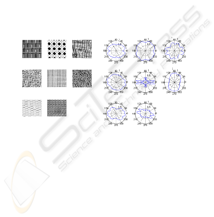
Fig. 1(a) shows texture samples from the textures used in the experiments. Fig.
1(b) shows polar plots of eight feature vectors, one vector sample from each of the
eight textures. In general, oriented energy feature vectors are periodic with period
360
o
. In this particular case where the filters used are anti-symmetric, feature extrac-
tion results in feature vectors with period 180
o
.
3.1 Percentage of Correct Clustering
In this work, the clustering performance is measured using the Percentage of Correct
Clustering (PCC) [14] defined as follows. Let l = 1, 2, …, L, be the index in a set of L
known labels, and l’ = 1, 2, …, L’ be the index that identifies the l’-th cluster out of
L’ clusters. A cluster l’ is labeled “l”, if the number of vectors labeled l, contained in
l’, is larger than the number of vectors, also contained in l’, labeled with any other
single label. Then, the PCC for cluster l’ is defined as:
PCC
1’
= 100 J
l
/ J
l’
(31)
where J
l
is the number of label l vectors in cluster l’, and J
l’
is the total number of
vectors in cluster l’. The overall PCC is defined as
∑
=
'
''
PCC
100
PCC
l
ll
J
J
(32)
39
where J is the total number of vectors. For this experiment, all possible combinations
of two, three, and four textures out of all eight textures are considered. The average
PCC is found in each case. Moreover, clustering using all eight textures is performed.
Texture 1 Texture 2 Texture
Texture 4 Texture 5 Texture
Texture 7 Texture 8
Since only the PCC is examined here, the number of clusters is assumed to be
equal to the ANC, which is equivalent to the number of textures from which feature
vectors have been obtained. Table 1 presents comparison results for three different
circular invariant approaches, namely the proposed CK-means algorithm, the original
K-means using the FFT magnitudes of the feature vectors [8], and the original K-
means using the maximum orientation-differences [9]. A maximum orientation-
difference feature is defined as the maximum value considering all vector element
differences for a given angular distance. In this example, angular distances of m⋅18
o
,
m = 1, 2, …, 5 are used. Small angular distances do not add significant information,
since they are expected to be small. Thus, a larger number of angular distances does
not necessarily add to the clustering performance.
Texture 1 Texture 2 Texture 3
Texture 4 Texture 5 Texture 6
Texture 1
Texture 7 Texture 8
Texture 2
Texture 3
Texture 4
Texture 5 Texture 6
Textur 7 e
Texture 8
Fig. 1. (a) Samples from the textures used for the clustering experiment. (b) Polar plots of
energy extracted in multiple orientations from a 64×64 block from each texture of Fig. 1(a).
In Table 1, different Cluster Ratios (CR) are used. For instance, 4|3|1 indicates
that the data set consists of vectors belonging to three clusters, one of which has 4
parts, another has 3 parts and the third has 1 part. Similarly, 1|1|1 indicates that the
number of vectors per cluster is the same for all three clusters. Table 1 illustrates that
CK-means provides accurate clustering results. More specifically, the proposed tech-
nique provides 3-5% or 2-9% higher PCC than the original K-means, where the FFT
magnitudes of the original vectors or the MODF - 5 features are used.
40
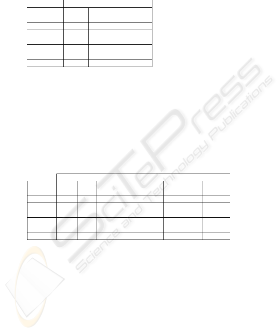
Table 1. Average percentage of correct clustering for three approaches.
Average PCC
ANC CR Proposed FFT-magn. MODF - 5
2 1|1 99.6% 96.7% 96.0%
2 2|1 99.7% 96.7% 94.3%
3 1|1|1 99.1% 96.3% 90.6%
3 4|3|2 99.6% 95.7% 90.1%
4 1|1|1|1 98.4% 94.7% 86.3%
4 4|2|1|1 98.8% 93.4% 91.6%
8 1|1|…|1 93.8% 90.6% 84.4%
3.2 Estimating the Actual Number of Clusters
This experiment is performed for the same set of eight textures, and the results are
presented in Table 2. Table 2 presents the average number of clusters, and the per-
centage of times each approach found: the correct ANC, one cluster different than the
ANC, and more than one clusters different than the ANC. Table 2 illustrates that the
proposed technique is mostly successful in identifying the correct number of clusters,
while when incorrect, it is mostly off by one cluster. On the other hand, the FFT-
magnitude approach is correct for a significantly less number of times, while it is
frequently off by more than one cluster.
Table 2. Statistics from the “Number of Correct Clusters” experiment for the proposed CK-
means clustering technique, and the original K-means using the vectors’ FFT magnitudes.
Proposed Algorithm Original K-means
ANC CR
Average
NC
Correct
NC
NC =
ANC±1
NC=ANC±h
h>1
Average
N
C
Correct
N
C
N
C=
ANC±1
N
C=ANC±h
h>1
2 1|1 2.00 100.0% 0.0% 0.0% 3.20 46.7% 13.3% 40.0%
2 2|1 2.00 100.0% 0.0% 0.0% 3.40 40.0% 13.3% 40.0%
3 1|1|1 2.89 78.6% 21.5% 0.0% 4.54 32.1% 25.0% 42.9%
3 4|3|2 2.88 57.1% 41.1% 1.8% 4.43 33.9% 23.2% 42.9%
4 1|1|1|1 3.87 61.6% 35.7% 2.9% 4.69 60.0% 27.2% 24.3%
4 4|2|1|1 3.61 42.9% 22.8% 14.3% 6.24 12.9% 24.3% 62.9%
4 Conclusions
This paper presents an algorithm based on K-means, namely CK-means, for circular
invariant vector clustering. In general, one of the problems associated to the need for
circular invariant clustering is that most feature vectors extracted from the images or
objects under consideration are not circular invariant. Thus, a feature vector trans-
formation which provides the desired invariance characteristic is required. In most
cases, such a transformation ignores some vector information. In this paper, it is
shown that eliminating such information is crucial.
41

On the other hand, the proposed CK-means performs clustering in a circular in-
variant manner without eliminating information from the original feature vectors,
other than the circular shift. Furthermore, CK-means is robust in terms of PCC and in
terms of estimating the Actual Number Clusters. Furthermore, the computational
complexity of CK-means is not significantly higher than that of K-means.
References
1. Jain A.K. and Dubes R.C.: Algorithms for Clustering. Englewood Cliffs, N.J. Prentice Hall,
(1988)
2. Duda R.O. and Hart P.E.: Pattern Classification and Scene Analysis. New York, Wiley,
(1973)
3. Bezdek J.: Pattern Recognition with Fuzzy Objective Function Algorithms. New York,
Plenum, (1981)
4. Hartigan J.: Clustering Algorithms. New York, Wiley, (1975)
5. Tou J. and Gonzalez R.: Pattern Recognition Principles. Reading, Mass., Addison-Wesley,
(1974)
6. Ruspini E.: A New Approach to Clustering. Information Control, Vol. 15, No. 1, (1969) 22-
32
7. Su M.C. and Chou C.-H.: A Modified Version of the K-Means Algorithm with a Distance
Based on Cluster Symmetry. IEEE Transactions on Pattern Analysis and Machine Intelligence,
Vol. 23, No. 6, June (2001)
8.
Arof H. and Deravi F.: Circular Neighborhood and 1-D DFT Features for Texture Classification
and Segmentation,” IEE Proceedings, Vision Image and Signal Processing, Vol. 145, No. 3,
(1998) 167-172
9. Charalampidis D. and Kasparis T.: Wavelet-based Rotational Invariant Segmentation and
Classification of Textural Images Using Directional Roughness Features. IEEE Transac-
tions on Image Processing, Vol. 11, No. 8, (2002) 825-836
10. Haley G.M. and Manjunath B.S.: Rotation-invariant Texture Classification Using a Com-
plete Space-Frequency Model. IEEE Trans. on Image Processing, Vol. 8, No. 2, (1999)
255-269
11. Cohen F.S., Fan Z., and Patel M.A.: Classification of Rotated and Scaled Textured Images
Using Gaussian Markov Random Field Models. IEEE Transactions on Pattern Analysis and
Machine Intelligence, Vol. 13, No. 2, (1991) 192-202
12. Gray R.M.: Toeplitz and Circulant Matrices: A Review. Web Address:
http://ee.stanford.edu /~gray/toeplitz.pdf
13. Charalampidis D., Kasparis T., and Jones L.: Multifractal and Intensity Measures for the
Removal of Non-precipitation Echoes from Weather Radars. IEEE Transactions on Geo-
science and Remote Sensing, Vol. 40, No. 5, (2002) 1121-1131
14. Georgiopoulos M., Dagher I., Heileman G.L. and Bebis G.: Properties of learning of a
Fuzzy ART Variant. Neural Networks, Vol. 12, No. 6, (1999) 837-850
42
