CONCEPTUAL OPTIMISATION IN BUSINESS PROCESS

MANAGEMENT

Yves Callejas, Jean Louis Cavarero, Martine Collard

Université de Nice-Sophia Antipolis, Laboratoire I3S

2000, route des lucioles, O6903 Sophia Antipolis cedex, France

Keywords: Business process management, quality, Modelling, evaluation, simulation, optimisation, linear and non

line

ar programming, activity diagrams, resources affectation.

Abstract: To optimise business processes is a very complex task. The go

al is double: to improve productivity and

quality. The method, developed in this paper, is composed of 4 steps : the first one is the Modelling step (to

describe the business process in a very rigorous way), then a conceptual optimisation (supported by

evaluation and simulation tools) to improve the business process structure (to make it more consistent, to

normalise it), then an operational optimisation to improve the business process performing (to make it more

efficient) by providing to each operation the necessary resources and at last a global optimisation (to take

into account all the business processes of the company under study). This method is the result of three years

research achieved for the French organism “Caisses d’Allocations Familiales: CAF”. It was validated on the

business processes of the CAF, which deal with information (files and documents), but it can also be applied

on industrial business processes (dealing with products and materials).

1 INTRODUCTION

Business process optimisation is one of the major

issues of any company. The main goals are to

improve processes quality and to improve their

productivity, by increasing the number of output

flows and/or by decreasing the quantity of necessary

resources [Rolland 1996, Butler 1999, Aalst 2002,

Aler 2002, Borrajo 2001, Estin 1996, Jonkers 1999,

Jensen 2001, Krajewski 2001, Drabble 2002,

Nareyek 2001, Haslum 2000, Williamson 1994].

The method presented in this paper starts with a

previous modelling step followed by three main

steps:

- the Modelling step

makes it possible to represent

BP with a model which has the usual guarantees of

any good model: readability, normalisation,

genericity, and which induces an optimisation more

rigorous, more consistent and less hazardous.

Modelling was decided for all these reasons in order

to avoid an empirical optimisation consisting in

improving each BP from clues based on its

behaviour, by trying to find out local solutions.

- the Conceptual optimisation step

which does not

take into account resources; it is a structural and

static optimisation.

- the Operational optimisation step

which consists in

optimising the performing of the BP by taking into

account resources, which means by locating them

the best way as possible. It is a dynamic

optimisation since the goal is to optimise

performances.

- the Multi-BP optimisation step

which is used to

optimise (in the operational way) several BP

simultaneously.

2 MODELLING

Four concepts are necessary to model business

processes: operation, flow, resources and

competencies.

Operations

: an operation is a task of a business

process. Each operation can be mandatory or

optional. A mandatory operation has to be used

systematically (always), which means it is necessary

for the right performing of the BP. An optional

operation may not be used depending on the decided

options.

Flows

: A flow is a set of homogeneous elements

passing through the BP and treated by operations.

An optional flow is a flow associated to an optional

operation. Resources and Competencies

: These 2

concepts are linked. A resource is a group of persons

having the same set of competencies. A resource

possesses one or several competencies. A

233

Xu D. (2005).

THREAT-DRIVEN ARCHITECTURAL DESIGN OF SECURE INFORMATION SYSTEMS.

In Proceedings of the Seventh International Conference on Enterprise Information Systems, pages 233-239

DOI: 10.5220/0002552002330239

 SciTePress

competency can be associated to several resources

(N: M link). The set of resources is a partition of the

persons set.

We consider that each operation is one-competency.

The chosen model is directly inspired from the UML

activity diagrams. In order to build activity

diagrams, we can use any tool supporting UML

notations. We can choose either a full UML

environment like RATIONAL ROSE or DESCRIBE

or a graphic modelling tool like VISIO or

SMARTDRAW. DESCRIBE was finally chosen,

because it is the tool which satisfy the better these

criteria.

3 OPTIMISING

The modelling step provides a diagram of the BP (by

using the previous concepts) in order to evaluate it

(with simulation and evaluation tools) and to

optimise it in the right directions.

3.1 Collecting information

3.1.1 Indicators

Indicators are used to evaluate a BP. They are of 2

kinds: model indicators and BP indicators.

Model indicators: they are used to evaluate the

consistency of a BP independently of its finality.

They are theorical indicators (in opposition to BP

indicators). They provide an evaluation of the

diagram quality and make it possible to check that

diagrams are satisfying the norms given by the

model. In others words, to check that the conceptual

optimisation step delivers well built

diagrams. Examples of model indicators are

following:

maximum number of input and output flows in each

operation, average number of flows per operation,

number of operations, number of loops, cyclomatic

number (number of bows-number of nodes + 2),

diagram density (number of bows/maximum number

of bows), average number of operations per

competency.

BP indicators: they are used to evaluate

performances and dysfunction of a BP. Their values

are useful to determine the optimisation priorities.

The modelling step and the objectives graph (see

Fig. 2) step make it possible to find out (for a given

BP) the list of the useful indicators.

Fig. 1 shows some examples of BP indicators in a

specific BP from the CAF

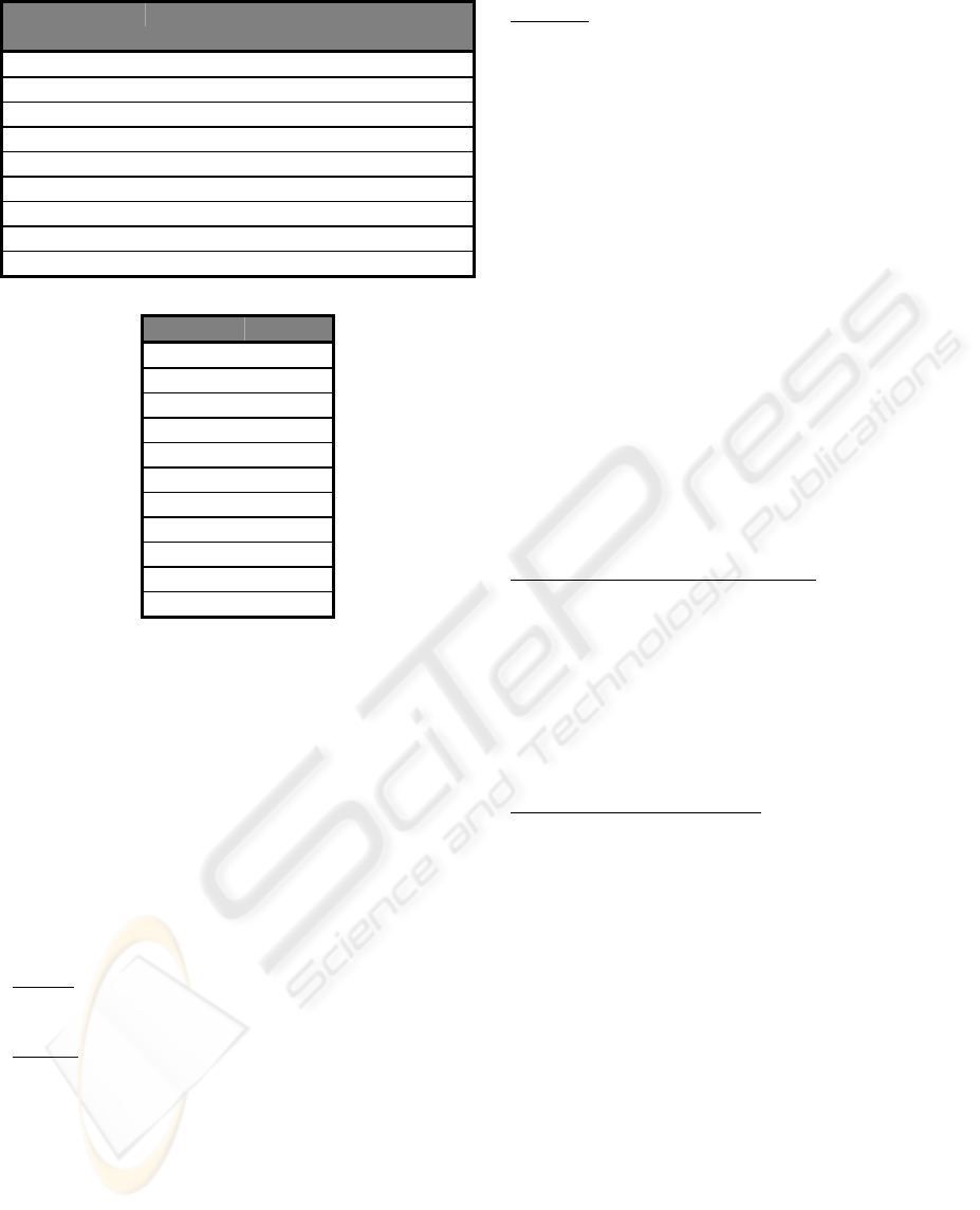
NODES OF THE GRAPH INDICATORS FORMAT WAY TO OBTAIN

READABILITY OF DOCUMENTS I1 : SATISFACTION PER DOCUMENT VECTOR OBSERVATION

DECREASE RATE REJECT I2 : % REJECT PER OPERATION VECTOR SIMULATION

DEMATERIALISATION I3 : % DEMATERIALISATION NUMBER OBSERVATION

Figure 1: Examples of BP indicators

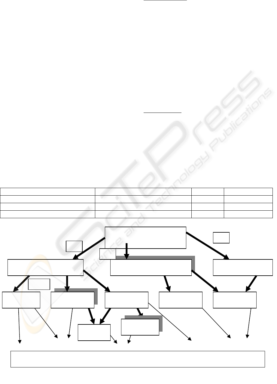
Improve Customer

Relationship (Root)

Decrease performing

Time of files

Increase documents

Readability I1

Decrease wrong

decisions

Decrease reject

Rates I2

Improve flows

Traffic

Better traduct

laws

Change some

Files

Increase

Performances

Improve

filters

Action 1

Action 3

Action 4

Action 5

P1+P2+P3=100%

P1*P11 is the weight of the objective “Increase performances” on the root objective

P11

Action 1

Dematerialise

Figure 2: Example of hierarchical objectives graph

ICEIS 2005 - INFORMATION SYSTEMS ANALYSIS AND SPECIFICATION

234

3.1.2 Hierarchical Objectives Graph

It is necessary to build a hierarchy of optimisation

objectives and to identify precisely those which are

means compare to the others. Thus, we propose to

build a “hierarchical objectives graph” (HOG). This

kind of graph makes it possible to show clearly the

hierarchical relationships between objectives.

If the graph is well built and exhaustive, all its

leaves are the actions to perform in order to optimise

the BP. More precisely, the graph is built by

connecting (if possible) to each node (objective)

some indicators, values of which will be provided by

evaluation and simulation steps (in the example I1,

I2 and I3).

The graph is helpful to build an optimise BP because

it gives the hierarchical links between objectives and

then optimisation priorities. Each BP has its own

graph. The bows of the graph have to be valuated

(with percentages) in order to give the satisfaction

weight of an objective to another one (higher in the

hierarchy) and to guide the process optimisation.

Simulation

This step is dedicated to the study of the BP

behaviour in order to find out some of the possible

improvements (addition or deleting operations

and/or flows, detection of wrong cycles, detection of

congestion points,…). Obviously, this step requires a

simulation tool (SIMPROCESS was chosen).

The simulation step is also used to give values to

indicators, such as the reject ratio per operation

3.2 Building the best BP

The conceptual optimisation of a BP is achieved

from information provided by evaluation step,

simulation step and objectives graph step. The goal

is to build the best BP as possible (in regards to

norms, indicators, objectives hierarchy). It is a very

tough step (totally hand made) which requires to

take into account simultaneously a very large

number of information and a great know how. Thus,

values of some model indicators will induce creation

or suppression of some operations and/or flows,

values of some BP indicators will generate creation

of some new paths in the diagram (by validating or

deleting optional operations) or creation of new

documents, analysis of the objectives graph make it

possible to identify the parts of the BP which have to

be optimised in priority.

Conceptual optimisation is totally guided by the

objectives graph: weights are used to know priorities

and indicators are used to decide if the nodes are

easy to optimise or not. In the example, we can

decide to give a priority to the objective “decrease

the time to perform a file” if the values of I2 are too

high and if the weight of this objective in regards to

the root objective is high. In this case, we have to

(following the graph) modify some resources and

add some operations. In opposition, if the value of I1

is too low and if the weight of the objective “to

increase readability of documents” is high, then we

have to design new documents.

Actually, the conceptual optimisation of a BP is

achieved by a lot of improvements (defined in the

leaves of the graph) performed on its diagram, in

regards to the objectives graph which gives the right

directions. But the diagram’s improvement has to be

done in respect of concepts. For this reason, we have

defined the exhaustive list of generic actions (meta-

actions) which are possible to do. Each leaf of the

graph has to be obviously an instance of one meta-

action.

Examples of meta-actions: to add a new operation,

to automate partially an operation, to split an

operation (in 2 or more) to add a new flow, to merge

2 or more flows into 1, to modify a flow, to add a

new competency, to change the destination operation

of a flow

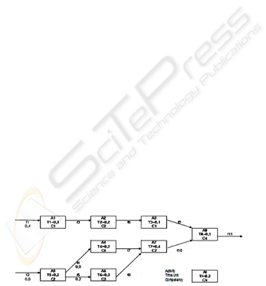
Figure 3: An example of BP

CONCEPTUAL OPTIMISATION IN BUSINESS PROCESS MANAGEMENT

235

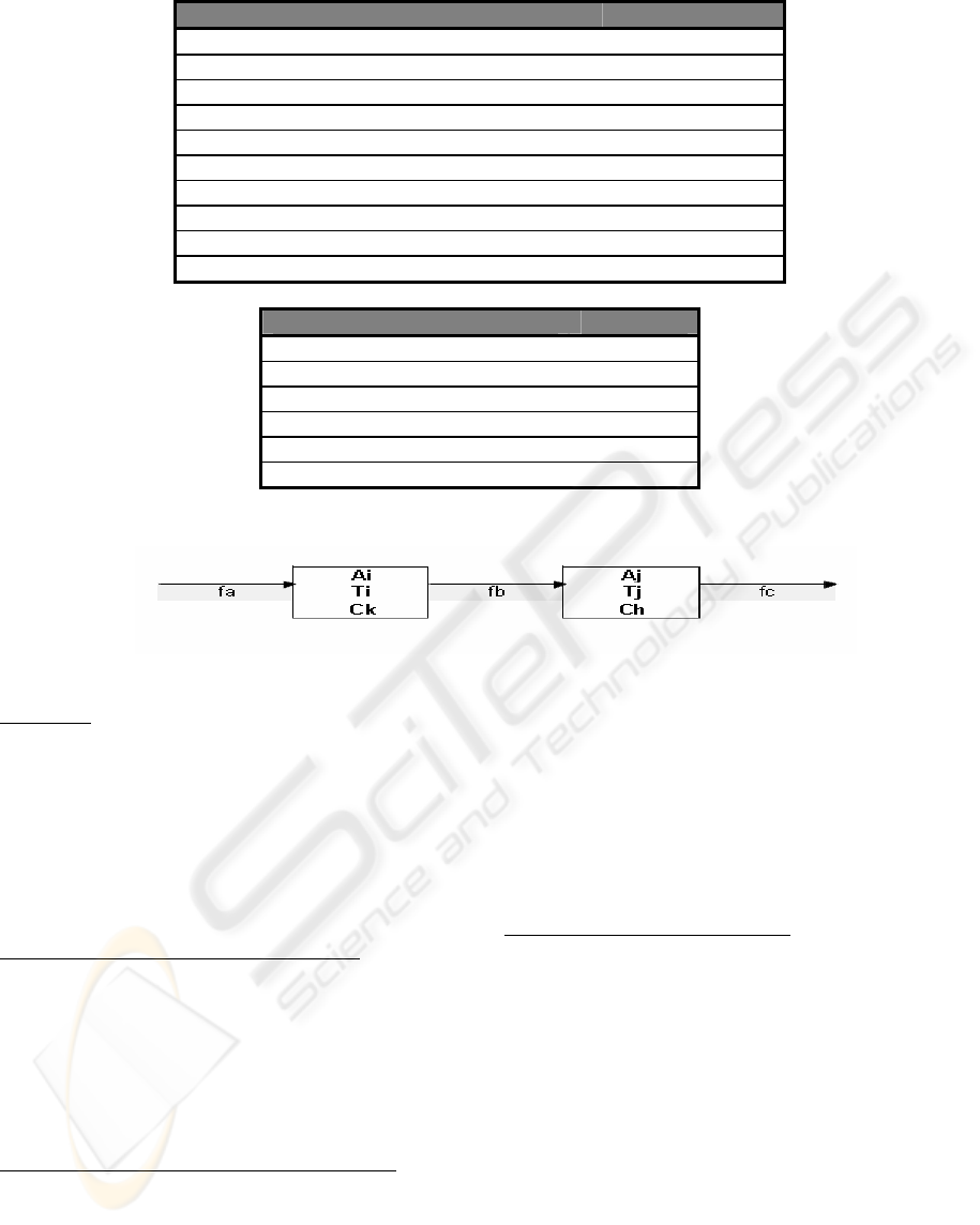
RESOURCE COMPETENCY AVAILABILITY/

PERIOD

R1 C2 TR1=35

R2 C1, C2 TR2=35

R3 C3 TR3=35

R4 C1, C4 TR4=35

R5 C4 TR5=35

R6 C2, C3 TR6=35

R7 C2 TR7=35

R8 C2 TR8=17.5

R9 C1 TR9=17.5

Figure 4: Table resources/competencies.

FLOWS STOCKS

f1 29

f2 58

f3 6

f4 2

f5 6

f6 4

f7 4

f8 2

f9 4

f10 8

f11 0

Figure 5: Table of flows stocks.

3.3 Predicting the best affectation of

resources

This step consists in giving to each operation of a

BP, resources and competencies, in order to

maximise output flows. Actually, the final goal is to

provide a command tool to predict the best resources

affectation as possible, by taking into account

different hypothesis of degraded performing (for

example absenteeism) as well as flows stocks (flows

which have not been treated).

This third step is divided in two distinct issues:

Issue 1: Searching optimum of outputs flows (by an

optimised affectation of resources and competencies

to operations (linear optimisation).

Issue 2: Locating resources and competencies on

each operation at the right time (non linear

optimisation).

To illustrate this step, let’s take an example of BP

given in Fig. 3.

This BP is composed of 8 operations (A1, A2,.., A8)

and 9 resources (R1, R2,…, R9). The relationships

between resources and competencies are given in

Fig. 4, the stocks of flows are given in Fig. 5. Let fp

be the number of units of flow p treated and wjk be

the used time of the resource Rj for its competency

Ck (during the chosen period).

Issue 1 consists in giving resources and

competencies to each operation (by finding out

optimal values of fp and wjk) (who does what?) and

in computing the maximum number of output flow

units. The equations system to solve is following; it

corresponds to using conditions of competencies on

the period.

Competency C1 T1*f3 + T3*f9 = w21 +

w41 + w91

Competency C2 T2*f6 + T5*(f4+f5) + T7*f10 =

w12 + w22 + w62 + w72 + + w82

Competency C3 T6*f8 = w33 + w63

Competency C4 T4*f7 + T8*f11 = w44 + w54

The first legs of these equations are the total used

time of competencies. For example, competency C1

which is used in operations A1 and A3 is engaged

for a time T1*f3 in A1 and T3*f9 in A3. The second

legs correspond to the used time of competencies in

regards to resources. For example, competency C1 is

provided for a time w21 by resource R2, for a time

w41 by resource R4 and for a time w91 by resource

R9.

To solve the system we also have to take into

account two types of constraints:

Availability constraints of resources:

For each resource Rj, total used time should not be

higher than available time. There are 9 constraints of

this kind:

R1: w12 ≤ TR1 R2: w21 + w22 ≤ TR2

R3: w33 ≤ TR3 R4: w41 + w44 ≤ TR4

R5: w54 ≤ TR5 R6: w62 + w63 ≤ TR6

R7: w72 ≤ TR7 R8: w82 ≤ TR8

R9: w91 ≤ TR9

Pouring constraints on flows: Input and output flows

can be multiple. To express that input flow f2 is

approximately 60% of the total input flow (f1+f2),

we write one constraint on the flow from f1 and on

the flow from f2: f2 ≥ 1.4 * f1 and f2 ≤1.6 * f1.

To express that output flow f4 is approximately 80%

of the total output flow (f4+f5), we write one

constraint on the flow from f4 and on the flow from

f5; we write a similar constraint on the flows f7 and

f8: f4 ≥3.9 * f5 and

f4 ≤ 4.1 * f5, f7 ≥ 3.9 * f8 and f7 ≤ 4.1 * f8.

For each operation, the sum of output flows has to

be inferior to the sum of input flows: f11 ≤ f9 + f10,

f9 ≤ f6, f6 ≤ f3, f3 ≤ f1, f10 ≤ f7 + f8, f7 ≤ f4, f8 ≤

f5, f4 + f5 ≤ f2

The solver provides values of fp and wjk which

optimise output flows. The results are given in the

next tables

ICEIS 2005 - INFORMATION SYSTEMS ANALYSIS AND SPECIFICATION

236

RESOURCE ∑

wjk AVAILABLE TIME

R1 w12 : 28 28 7

R2 w21 : 10.5 w22 : 21 31.5 3.5

R3 w33 : 17.5 17.5 17.5

R4 w41: 3.5 w44 : 31.5 35 0

R5 w54 : 21 21 14

R6 w62 : 28 w63 : 3.5 31.5 3.5

R7 w72 : 31.5 31.5 3.5

R8 w82 : 17.5 17.5 0

R9 w91 : 17.5 17.5 0

TOTAL 231 49

Figure 6: Table of competencies used time

Input flows

f1 95

f2 176

Stocks 123

Total (input + stocks) 394

Output flows (f11) 280

Non treated flows 114

Figure 7: Flows results

Figure 8: Evolution of flows

Issue 2 consists in searching dated resources

locations. (Who does what and when?). For this

reason, we have to split the period (35 hours in the

example) in 10 slices of same length D (3,5 h in the

example), and we have to find out quantities of

resources to give to each operation in each slice. The

result will be the used resources and competencies

for each slice.

For this issue, the system solving has to take into

account 3 types of constraints:

Exclusivity constraints on competencies. For each

multiple competency resource, at most one

competency is used in each slice. As we have 9

resources and 10 slices, we have 90 constraints of

this kind. If we name{Cjk}

k∈ 1..p

the set of

competencies associated to resource Rj, the

constraint may be expressed in the following way:

∀ (Resource Rj, slice t) ∃ at most one k ∈ 1..p such

that Cjk is used in slice t.

Using constraints of resources in operations. They

are equality constraints. For each slice and for each

competency, there is equality between quantities of

competencies used by operations and quantities of

competencies taken in resources. In the example,

there are four competencies and 10 slices; we have

then 40 constraints of this kind.

If we name {aik(t)}

k∈ 1..p

the set of used times of

competency Ck for the operation Ai on the slice t

and {w’jk(t)}

k∈ 1..q

the set of used times of resource

Rj for its competency Ck on the same slice, the

constraint may be expressed in the following way:

∑

aik(t) = ∑

w’jk (t) where aik(t) = αik(t) * D ;

αik(t) representing the number of times competency

Ck is used for operation Ai on the slice t (that is the

number of used resources).

Evolution constraints on flows. We assume that

flows evolve in a discontinuous way. After each

slice, flows evolve in regards to resources provided

to operations and available flows of the previous

slice. Let’s take a basic example of Fig. 8.

The formula which gives flow fb after slice t is:

Flux(b,t) = Flux(b,t-1) + Min(Flux(a,t-1),

αik(t)*D/Ti) - Min(Flux(b,t-1), αjk(t)*D/Tj) where

αik(t) represents the number of times competency

Ck is used for operation Ai on the slice t.

It is necessary to adapt this formula if operation Ai

or Aj are preceded and/or followed by several

operations.

An additional table is used to give quantities of input

flows on each slice (in regards to the chosen arrival

law)

CONCEPTUAL OPTIMISATION IN BUSINESS PROCESS MANAGEMENT

237

OPERATION S1 S2 S3 S4 S5 S6 S7 S8 S9 S10 COMPETENCY

A1 1 0 1 0 0 1 0 0 0 0 A1

A2 0 1 0 0 0 1 3 1 0 0 A2

A3 0 0 0 0 1 1 0 2 2 0 A3

A4 0 1 1 1 1 2 1 0 0 0 A4

A5 3 3 5 0 0 0 0 0 0 0 A5

A6 0 0 1 2 1 1 0 1 0 0 A6

A7 0 0 0 4 5 3 1 3 3 0 A7

A8 0 0 0 0 1 0 1 2 2 2 A8

Figure 9: Table of competency/operation affectation for each slice

The solver provides values of αik(t) which optimise

the repartition of resources and competencies on

each sliceand associated flows.

The table of Fig. 9 shows, the number of times αik(t)

competency Ck is used for operation Ai for the slice t. For

example, on the first slice, three resources of competency

C2 are given to operation A5 and on the fourth slice two

resources of competency C3 are given to operation A6.

4 MULTI-BP OPTIMISATION

As indicated by its name, multi-BP optimisation

consists in optimising simultaneously several BP.

Obviously, this step does not involve conceptual

optimisation (which is, by definition, made on one

BP, independently from the others) but only

operational optimisation in the case where resources

and competencies are shared by several BP. If so,

the persons in charge of the business processes have

to define priorities between BPs and constraints on

resources and competencies which will be given to

BPs and operations.

When priorities and constraints are defined, the

solver can be run (one to N times) by deleting one

by one constraints (from the bottom of the list) while

objectives are not satisfied. The multi-BP

optimisation step is, thus, a generalisation of the

operational optimisation step, using the same tool

and being done several times in a row. The final goal

is to achieve a full and global command of all the

BPs of the company

5 CONCLUSION

The optimisation method presented in this paper is

composed of 4 steps: Modelling step, conceptual

optimisation step, operational optimisation step,

multi-BP optimisation step. Its originality consists in

separating clearly issues related to modelling and

issues connected to optimisation. The first step

(Modelling step) is necessary to model BPs under

study and so necessary for the 3 others steps. The

second one (conceptual optimisation step) make it

possible to build the best BPs as possible, consistent

and normalised (in regards to norms, objectives and

indicators). The third one (operational optimisation)

is probably the main one. Its goal is to improve the

performances and behaviour of BPs by optimising

resources and competencies locations.

This method was validated on administrative BPs. It

also works on industrial BPs, under condition to take

into account (during the operational optimisation)

issues of breakdowns and maintenance of machines

(by using complementary tools), issues which were

not presented in this paper. This research is going to

be extended by introducing data mining techniques

in the conceptual step in order to find out more

efficient optimising rules. We would like to thank

the CNEDI 06 and more particularly M.P. Bourgeot

who made this research possible

REFERENCES

Aalst, W. and Hee, K.V, 2002. Workflow

Management: Models, Methods, and Systems,

ISBN : 0-262- 1189-1, MIT Press.

Aler, R. Borrajo, D. Camacho, D. and Sierra-

Alonso, A. , 2002 A knowledge-based approach

for business process reengineering, SHAMASH.

Knowledge Based Systems, 15(8):473–483.

Borrajo, D. Vegas, S. and Veloso, M., 2001. Quality

based learning for planning. In Working notes of

the IJCAI’01 Workshop on Planning with

Resources, pages 9–17, Seattle, WA (USA),

IJCAI Press.

Drabble, B. Koehler, J. and Refanidis, I. editors,

2002. Proceedings of the AIPS-02 Workshop on

Planning and Scheduling with Multiple Criteria,

Toulouse (France).

Estlin, T.A and Mooney, R.J., 1996. Multistrategy

learning of search control for partial-order

ICEIS 2005 - INFORMATION SYSTEMS ANALYSIS AND SPECIFICATION

238

planning. In Proceedings of the Thirteenth

National Conference on Artificial Intelligence,

volume I, pages 843–848, Portland, Oregon.

AAAI Press/MIT Press.

Haslum, P. and Geffner, H., 2000. Admissible

heuristics for optimal planning. In Proceedings

of the Fifth International Conference on AI

Planning Systems (AIPS-2000), pages 70–82.

Jensen, P.A and Bard, J.F., 2001.

Operations

Research Models and Methods

, ISBN : 0-471-

38004-0, Wiley Higher Education

Krajewski, L. and Ritzman, P., 2001. Operations

Management: Strategy and Analysis (6th

Edition), Prentice Hall, London, 2

edition.

Nareyek, A. editor, 2001. Working notes of the

IJCAI’01 Workshop on Planning with Resources,

Seattle, WA (USA), IJCAI Press.

Williamson, M and Hanks, S., 1994. Optimal

planning with a goal-directed utility model. In K.

Hammond, editor, Proceedings of the Second

International Conference on Artificial

Intelligence Planning Systems (AIPS94), pages

176–181, Chicago, Illinois

CONCEPTUAL OPTIMISATION IN BUSINESS PROCESS MANAGEMENT

239