
A THEORETICAL PERFORMANCE ANALYSIS METHOD FOR
BUSINESS PROCESS MODEL
Liping YANG, Ying LIU, Xin ZHOU
IBM China Research Lab
Keywords: Computational Model, B
alance Equation System, Bottleneck, Business Process Model
Abstract: During designing a business process model, to predict its performance is very important. The performance
of business operational process is heavily influenced by its bottlenecks. In order to improve the
performance, finding the bottlenecks is critical. This paper proposes a theoretical analysis method for
bottleneck detection. An abstract computational model is designed to capture the main elements of a
business operational process model. Based on the computational model, a balance equation system is set up.
The bottlenecks can be detected by solving the balance equation system. Compared with traditional
bottleneck detection methods, this theoretical analysis method has two obvious advantages: the cost of
detecting bottlenecks is very low because they can be predicted in design time with no need for system
simulation; and it can not only correctly predict the bottlenecks but also give the solutions for improving the
bottleneck by solving the balance equation system.
1 INTRODUCTION
In order to keep competitive in the marketplace,
enterprises have to continuously increase the
performance while reducing the cost. Business
process modeling represents the business logic of an
enterprise’s business activities. It includes mainly
three kinds of important components: activities, data
processed by activities and resources allocated to or
consumed by activities. Performance of business
processes running in an enterprise influences heavily
on performance of the whole enterprise. As a result,
it is effective to improve enterprise performance by
accelerating its business processes.
A large number of experiences accumulated in
business
practice indicate that keeping compatible
data processing speed of relative activities and
appropriate allocation of resources are two major
factors for high performance. Otherwise,
performance bottlenecks constraint the whole
process performance. Given a manufacturing
enterprise that has a high-speed producing
department and a low-speed sales department, it will
have to stop operating due to the overflow
warehouse sooner or later. Once the root cause
behind this phenomena is detected, the enterprise
can adjust the produce-store-sale process to gain the
producing speed, sales speed and warehouse
capacity suited by re-allocating resources. However,
detecting business process bottlenecks is usually
time consuming and prone to be inaccurate because
of the complexity of business process and the
inherent hidden characteristics of bottlenecks.
Therefore, an effective and accurate approach is
urgently needed to detect the bottlenecks in business
process for performance improvement.
There are currently a lot of methods in use to detect
th
e bottlenecks(Christoph, 2003)(Christoph, 2001)
(Blake, 1995)(Lawrence, 1995). Two frequently
used methods are measuring waiting time and
calculating the utilization. Waiting time method is to
look for the machine where the parts have to wait for
the longest time. A common method is to look for
the longest queue. However, this approach works
only for linear systems containing only one type of
part. The utilization based method is to measure the
percentage of the time that a machine is active, and
then define the machine with the largest active
percentage as the bottleneck. Both of these two
approaches have several drawbacks.
For measuring waiting time, the accuracy of this
approach is c
ompromised if the system contains
73
YANG L., LIU Y. and ZHOU X. (2005).
A THEORETICAL PERFORMANCE ANALYSIS METHOD FOR BUSINESS PROCESS MODEL.
In Proceedings of the Seventh International Conference on Enterprise Information Systems, pages 73-80
DOI: 10.5220/0002537700730080
Copyright
c
SciTePress

buffers of limited size. Furthermore, this approach
analyzes only the processing machines of the
manufacturing system. Other elements, such as
human workers, supply and demand, do not have the
concept of buffer, so that the waiting time measuring
approach is not feasible for them. For measuring
utilization, the measure result may be not accurate
enough to be trusted because the difference between
the utilizations of the machines may be very small.
While this method is easy to be automated, the
results are not always accurate (Luthi, 1997).
Moreover, most of utilization bottleneck detection
methods are based on analyzing the system data in
running time or simulating the systems, which will
result in great cost and time consuming.
In this paper, an abstract computational model is put
forward aiming at analyzing business process
performance effectively and efficiently. Firstly, a
computational model is proposed to abstractly model
business process as sets of transitions, data, data
buffers, and connections between transitions, based
on which most of the common performance related
problems are described. Then, the problem of
analyzing bottleneck transitions in a business
process is theoretically induced as a Balance
Equation solving problem and a solving algorithm
for Balance Equation is proposed. Finally, real
business performance problems are analyzed using
above theoretical method to illustrate the application
of this approach and verify its effect.
We start presenting the computational and analytical
model in Section 2. Section 3 introduces the
theoretical foundation, Balance Equation System, for
business transition bottleneck detection and proposes
the equation solving algorithm. Performance
problems in real case are dealt with in Section 4 for
illustrating and verifying the whole approach.
Section 5 concludes this paper and gives direction of
the future works.
2 THE COMPUTATIONAL
MODEL
To perform performance analysis, it’s necessary to
firstly abstract the system as a mathematical model.
Such mathematical models keep critical elements
but eliminate those unnecessary details. As a result,
we can focus on the perspective closely related to
the problem we concern. At the same time, we can
utilize some mathematical mechanism to detect the
bottleneck conveniently and accurately. A lot of
theoretical models can act this role, for example,
queue network(Donald, 1998), Petri Net(Ajmone,
1984)(Baccelli, 1993)(Salimifard, 2001), fluid
model(Kelly, 2004) etc. However, all these models
are not specially designed for analyzing the
performance of business process model. They are
complex and not easy to be used in the business
process bottleneck detection.
To simulate the behavior of a business process and
support further mathematical performance analysis,
we use a computational model defined in Definition
2.1. In our definition, four kinds of elements are
taken into consideration: transitions, data,
connections and data buffers. Transitions are
abstraction of activities in a business process, which
perform data processing in a certain period of time.
Data are abstraction of business items processed by
business process activities. The basic unit of data is
a data particle, which can be a group of transaction
data with fixed composition structure in a business
process. A connection is a directed linkage between
two transitions representing that output data from the
source transition provides input data for the target
transition. A data buffer is associated with a
connection to cache data for dealing with the run
time un-synchronization between two connected
transitions. A transition is periodically executed on a
fixed time interval. In case that one of the input
buffers is empty or an output buffer is full, the
current transition operation is skipped. Later, after
the time interval, the transition engine will come
again to see if the transition can be performed.
Definition 2.1 A Computational Model is a tuple (T,
C, B, Start, End, I/O, V
R
, V
E
), where,
1) T is a set of transitions. 2)C is a set of connections
that connect two transitions. 3)B is a set of data
buffers. Each data buffer may store multiple data
particles. 4)Start is a set of initial data buffers, and
the size of these buffers is supposed to be infinite.
5)End is a set of final data buffers, and the size of
these buffers is supposed to be infinite. 6)I/O is a
finite set. Each of the elements in the set is called a
data input/output structure (D-I/O-S) which is
defined for an individual transition. A D-I/O-S is
denoted as the following form: T
i
: ( ) -> (
N
ˆ
M
ˆ
ˆ
),
where T
i
is the transition, is the consumed data
particles by transition X, and
N
M
ˆ
is the produced
data particles. For example, T
1
: (1,2,2) -> (3,4)
means that each time transition T
1
consumes three
types of data particles and the number of each type
separately is 1, 2, and 2, and produces two types of
data particles and the number is 3 and 4. 7) V
R
is a
set of running speeds of all the transitions. 8) V
E
is a
set of effective speeds of all the transitions.
ICEIS 2005 - INFORMATION SYSTEMS ANALYSIS AND SPECIFICATION
74
For a transition, there are two important concepts
regarding its performance analysis: the running
speed V
R
of a transition and the effective speed V
E
of a transition. V
R
indicates the speed that the
transition accesses the input buffers in order to
perform an operation, i.e., the number of times that
the transition accesses the input buffers trying to
extract data particles from them within a time unit. It
should be noticed that not every attempt to extract
data particle can be accomplished. An attempt may
fail due to empty input buffer or fill-up output buffer.
V
E
indicates the speed that the transition accesses
the input buffers, gets data particles successfully,
and performs data processing, and writes data into
output buffers. From the definition, it obviously
holds V
R
≤
V
E
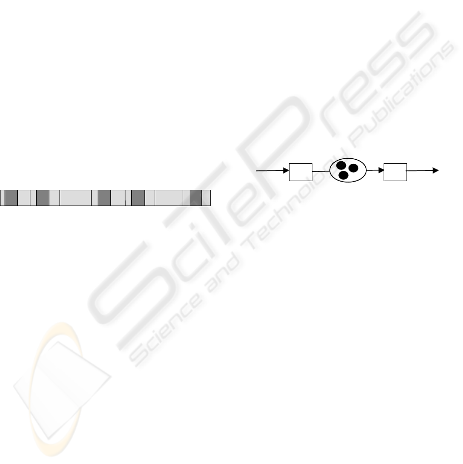
Figure 2.1 shows the status of a running transition.
In which the light-grey blocks indicates the pace of
running, while the dark-grey blocks show the pace
of processing. For the yellow block with red one in
it, that is the case that the operation fails to meet the
requirement for performing a transformation. The
ratio V
R
/V
E
represents the power usage of the
transition. The above two speeds are about the
average running speed. In the real world situation,
these speeds may vary with time.
Choice transition is a special kind of transition as
denoted in Figure 3.2. It is used to represent multiple
output choices for a transition. For the transition A,
there are three possible output paths connecting with
different next transitions. The transition C in the
diagram is the choice node. It is associated with
some judgment criteria in order to decide which
connection the data should move with. It should be
noticed that there is no buffer over the A-C
connection. This is because a choice node is treated
as a kind of super fast transition unit, such that every
input data will be passed to the next level
connections with no time delay.
3 THEORETICAL ANALYSIS
METHOD
The essential capability of process model is to
specify the behavior of a real business process. An
individual transition represents a behavior of a
business activity, and the execution logic of a set of
transitions is used to capture the behavior
environment of a business process. The performance
of a business process can be scaled by different
approaches, such as throughput of an activity and
task waiting time. In this paper, data throughput is
regarded as a performance scale standard for a
business process. That it to say, the more data is
manipulated within a time unit, the higher
performance of the business process will be.
For a business process, the execution logic structure
of its activities is usually known, which indicates
that the data input/output capability of each activity
in the process is known. This structure is defined as
data input/output structure of computational model.
Based on the above conditions, we can analyze the
global performance of the process model, so that the
analysis result can help design the running speed of
each activity and the size of every data buffer. In
order to analyze the performance of process model,
we designed a balance equation system (BES).
Based on BES, a lot of performance related business
problems can be solved.
3.1 Balance Equation System (BES)
C
A B
Figure 3.1 Sequential Structure.
Figure 3.1 is a simple Computational Model with
sequential execution logic. It includes two
transitions, A and B, and a data buffer C. The data
input/output structure of transition A is A: (N
XA
)-
>(M
AB
), and the data input/output structure of
transition B is B: (N
AB
)->(M
BY
). Suppose the
running speed of transition A and transition B
separately are V
A
and V
B
. For data buffer C, when
transition A puts V
XA
*M
AB
particles into the buffer,
transition B will extract V
AB
*N
BY
particles from the
buffer in the same time unit. In order to guarantee
the process can be safely and normally executed in a
long time, the V
A
*M
AB
and V
B
*N
BY
must be equal.
Otherwise, the buffer C will produce two situations:
one is the process is blocked because the buffer C is
full; and the other is transition B is idle because the
buffer is empty. The following is called Balance
Equation for buffer C:
Figure 2.1: Status of a running transition
V
A
M
AB
= V
B
N
AB
,
Where 0
≤
V
A
≤
U
A
and 0
≤
V
B
≤
U
B
(3.1)
Where, V
A
and V
B
are the effective speeds of
transition A and B respectively; U
A
and U
B
are the
upper bounds of V
A
and V
B
respectively. At the
design time of a model, U
A
and U
B
are parameters
for consideration. In the run time, U
A
and U
B
should
A THEORETICAL PERFORMANCE ANALYSIS METHOD FOR BUSINESS PROCESS MODEL
75

be
and respectively.
R
A
V
R
B
V
Figure 3.2 is a Computational Model with a choice
execution logic. The data input/output structure of
transition A is A: (N
XA
)->(M
AC
), and the data
input/output structure of transition B
i
(i=1, 2, 3) is
denoted as B
i
: (N
ABi
)->(M
BiY
)
.
So the Balance
Equation is as following:
ii
ABBAAi
NVMV =
α
3,2,1
=
i (3.2)
1=
∑
i
i
α
(3.3)
The above Balance Equations describe the basic
feature of the data particle flow over the
computational model. All the balance equations of a
computational model is called the Balance Equation
System of the model.
Properties: The following are some basic properties
of the balance equations.
1) There are exactly two non-zero elements
for each equation.
2) V=0 is a solution.
3) The solution set is convex.
In most cases, it holds in the model that the number
of connections is larger than the number of
transitions. This indicates that the BES is usually
over constrained.
Definition 3.1: The computational model is called
consistent if there is a non-zero solution for its BES.
3.2 Solvability of the BES
For any Balance Equation, we are going to study
what is the condition that it has non-trivial solution.
In order to give a general conclusion, an example is
used to illustrate the main idea. Figure 3.3 is an
example of Computational Model. It includes four
transitions, four data buffers, and four connections.
From transition A to transition B, there are two
paths, A-C-B and A-D-B.
The data input/output structures of transition A, B,
C, D separately are:
A: (N
XA
)->(M
AC
, M
AD
);
B: (N
CB
, N
DB
)->(M
BY
);
C: (N
AC
)->(M
CB
);
D: (N
AD
)->(M
DB
)
(MAC, MAD) denotes that transition A outputs data
MAC and MAD in parallel. MAC is for path A-C,
and MAD is for path A-D. (NCB, NDB) denotes that
transition B can be executed only accepting two
inputs from two paths in parallel. NCB is from C-B,
and NDB is from path D-B. The balance equation
system of this computational model is given as
following:
V
A
M
AC
= V
C
N
AC
(3.4)
V
C
M
CB
= V
B
N
CB
(3.5)
V
A
M
AD
= V
D
N
AD
(3.6)
V
D
M
DB
= V
B
N
DB
(3.7)
From the above balance equations, the following
two equations can be gotten:
BCBACCACA
VVV
α
α
α
=
=
(3.8)
BDBADDADA
VVV
α
α
α
=
=
(3.9)
, where α = N/M is called transforming parameter of
transition X and transition Y, and N is the data input
of transition Y, and M is the data output of transition
X. Comparing (3.8) and (3.9), we can get the
consistency condition for equations (3.4)-(3.7) to
have non-zero solution as:
DBADCBAC
α
α
α
α
=
(3.10)
Definition 3.2: Given a path in the computational
model, T
1
->T
2
->…->T
L
, the transforming
parameters of this path are defined as
αi =
∏
i
i
i
M
N
1+
(i=1, 2, …, L),
C
4
C
3
C
2
C
1
C
A
B
D
Figure 3.3: Computational Model Example
A
B2
Figure 3.2: Choice Structure
C
B1
B3
ICEIS 2005 - INFORMATION SYSTEMS ANALYSIS AND SPECIFICATION
76
where Ni+1 is data input of transition T
i+1
, and M
i
is
the output data of transition T
i
.
From the above example analysis, the following
theorem is easy to be understood.
Theorem 3.1: The BES has non-trivial solution if
and only if that for any two connected nodes on the
model, all the paths connecting the two nodes have
the same transition parameter.
Example 3.1: For the computation model in Figure
3.3, suppose its data input/output structure has the
following two situations, and the running speed of
every transition is (A,B,C,D)=(1,1,1,1):
A: (1)->(2,1); B: (1,1)-> (1);
C: (1)-> (1); D: (1)-> (1)
A: (1)->(2,1); B: (1,1)-> (1);
C: (1)-> (2); D: (1)-> (1)
For situation (1), the balance equation system is as
following:
2V
A
= V
C
V
A
= V
D
V
C
= V
B
V
D
= V
B
Obviously, it has no solution for these equations.
The transforming parameters of path A-C-B are
2
1
*
1
1
, and the transforming parameters of path A-
D-B are
1
1
*
1
1
. These parameters are not the same.
For situation (2), the balance equation system is as
following:
2V
A
= V
C
V
A
= V
D
V
C
= V
B
2V
D
= V
B
Then, we can solve the solution vector: (VA, VB,
VC, VD) = λ(0.5, 1, 1, 0.5), where 1 ≥ λ ≥ 0.
Similarly, we can get the transforming parameter of
path A-C-B as
2
1
*
1
1
, and
1
1
*
2
1
is the transforming
parameter of path A-D-B. Their parameters are the
same.
Theorem 3.1 gives the theoretical statement on the
feasibility of a computational model, which is the
very fundamental rule for designing a computational
model. In fact, a model with trivial solution is
equivalent to that the model can not run safely in a
long time. The above analysis on the transition
parameter also tells the following result.
Lemma: For any two nodes A and B in the model, if
they are connected and the BES has non-trivial
solution V, then the value V
A
/V
B
is a constant which
is independent of different solutions of the system.
Theorem 3.2: If every two nodes on the model is
inter-connected, then the solution for BES is unique
in the sense that for every two solutions there is a
constant C ≥ 0, such that V
1
= CV
2
.
Based on theorem 3.2, the vector
VVV =
∧
is denoted
as the unit solution of the BES.
Proposition: If the model is connected, it holds Vi >
0 for all i=1, 2, n, where V is a non-trivial solution
for BES.
3.3 Algorithm for Solving BES
Algorithm for solving BES
INPUT:
the transition number is n of this computational model;
data input/output structure T
i
: (N
i
)->(M
i
);
the running speed of every transition T
i
is U
i
;
N is the number of transitions in the computational
model;
OUPUT:
effective running speed V
i
of every transition T
i
Begin
for i=1,2,…N
initialize the value by setting V
i
= U
i
endfor
while ( there is a V
i
changed ) do
for i = 1, 2,…,N
for j = 1, 2,…N
if ((Connection(Ti,Tj) and (V
j
M
ij
< V
i
N
ij
))
then
Δ
V
i
= (V
i
N
ij
-V
j
M
ij
) / N
ij
V
i
=V
i
-
Δ
V
i
// such that V
j
M
ij
= V
i
N
ij
endfor
for k = 1,2,…N
if ((Connection(Ti,Tj) and (V
i
M
ik
> V
k
N
ik
))
then
Δ
V
i
=( V
i
M
ik
- V
k
N
ik
) / M
ik
V
i
=V
i
-
Δ
V
i
// such that V
i
M
ik
= V
k
N
ik
endfor
endfor
endwhile
Return V
End
Figure 3.4: BES Solving Algorithm
.
A THEORETICAL PERFORMANCE ANALYSIS METHOD FOR BUSINESS PROCESS MODEL
77

The algorithm in Figure 3.4 is an iterative one which
will solve the BES. In the algorithm, Vi indicates the
effective speed of the i-th node in the model. For a
given node, Vj is the speed of its j-th input node, and
Vk is the speed of its k-th output node.
In this algorithm, if a Vi converges to zero, which
indicates all of Vi converges to zero, then the model
does not have a non-trivial solution. During the
computation process in the above algorithm, VM
and VN is monotone descending, therefore, Δ Vi ≥ 0
and Δ Vi ≥ 0. If a Vi keeps unchanged during the
whole process of the algorithm, then this Vi is a
bottleneck node for the model.
3.4 Bottleneck Transition Analysis
In the equation (3.1), each variable V
i
has an upper
bound U
i
. In the language of computational model,
V
i
is the effective speed of the transition T
i
and U
i
is
the running speed of it. Each solution
V
for the BES
represents a group of steady solution for the
performance of transitions on the model. If the
effective speed of a transition is the first one to
approach to its upper bound while others remain
below their upper bounds, this transition is called the
bottleneck of the system. It is possible that a system
has more than one bottleneck.
Using theorem 3.2, the problem of finding the
maximum system performance becomes the problem
of solving
λ
from following equation,
(3.11)
)(max
max
= VV
λ
λ
∧
λ
0
, where
is used to dented the solution vector of a
BES is a solution of a BES, and λ ≥ 0, so
that
∧
.
^
V
i
i
UV ≤≤
Suppose
0
λ
is a constant which can be applied to
(3.11). From above analysis, we can get that the
bottleneck transitions for the computational model
are those transitions T
i
such that
(3.12)
i
i
UV =
0
λ
∧
When the model is running at its maximum
performance, only the transitions satisfying (3.12)
can reach its maximum performance such
that
E
i
R
. For other transitions, it
holds
. The power usage rate of transition T
i
VV =
E
i
R
i
VV >
i
i
i
i
U
V
=
0
λ
ρ
∧
(3.13)
From (3.13), it can be seen that only the bottleneck
nodes can reach their maximum power usage. For
example 3.1, if its data input/output structure is
situation (2), its bottlenecks have two transitions, B
and C, because their utilizations are the highest.
At the run time of the model, if all of the bottleneck
nodes are the input and output nodes, it indicates
there is potential to improve the performance of
system by improving the IO performance only.
Otherwise, improving the system performance will
have to depend on better system node performance
or better system structure.
4 APPLICATIONS OF
BOTTLENECK DETECTION
In real situation, there are a lot of business problems
caused by bottlenecks. However, these problems in a
real business process usually fall into some patterns.
In this section, we focus on two major patterns:
Input Data Flush pattern and Block Caused by a
Paused Transition pattern, and analyz them based on
the solution given above.
4.1 Analyzing Input Data Flush
In real business world, the volume of data input to a
business process varies from time to time and
usually large numbers of data suddenly flush into for
processing. We classify this kind of pervasive
running status as a pattern called Input Data Flush
pattern. For a business process in this pattern, it
really suffers from sudden flush of input data which
results in buffer jam, transition breakdown, and so
on. So it’s necessary to analyze and predict the
impact of flush input data and suggest some
approaches to counteract the negative effect. The
theoretical method proposed in Section 3 can be
leveraged to fulfill this demand.
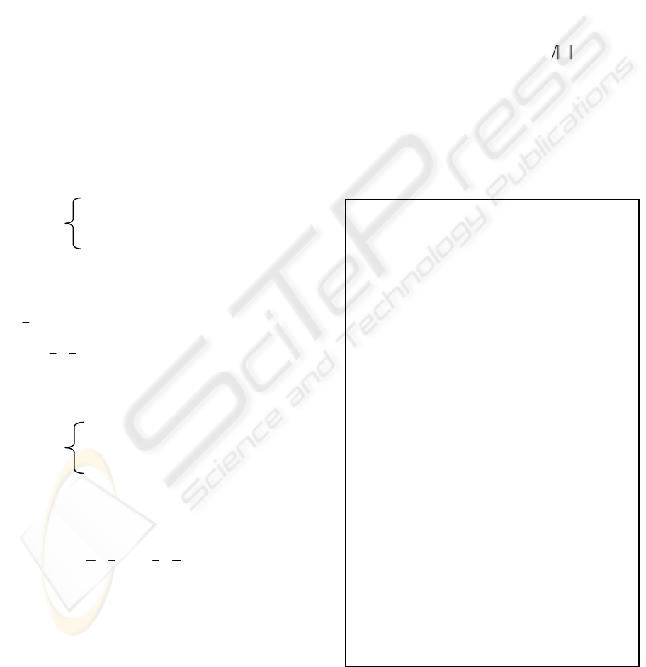
Given a business process represented in
computational model as shown in Figure 4.1, and
suppose we have detect the bottleneck transition T
i
by solving the Balance Equation System of such
process, we can predict the operation behavior of
each transitions as below:
If transition T
j
is a subsequent transition of T
i
and
there is a path from T
i
to T
j
, then T
j
will be light-
load transition sooner or later since low performance
Ti will limit the input data volume of T
j
.
ICEIS 2005 - INFORMATION SYSTEMS ANALYSIS AND SPECIFICATION
78
If transition T
j
is a previous transition of T
i
and there
is a path from T
j
to T
i
, then firstly T
j
will be heavy-
load transition due to large input volume but
gradually slow down because of buffer jams on the
path from T
j
to T
i
.
There is another critical issue to be analyzed for this
pattern. If one trying to accelerate the bottleneck
transition Ti for better process performance, it seems
wonderful but in fact dangerous if no deep analysis
and extra step are taken. Given there is a high
performance transition T
i+1
that is the direct
subsequent transition of T
i
, the performance of T
i+1
is prevented from full release by bottleneck
transition Ti before T
i
’s acceleration, then the low
performance transitions after T
i+1
can run safely
without worrying about buffer jam. However, once
we accelerate T
i
, then T
i+1
can fully release its
performance and buffer jam might produce between
T
i+1
and its low performance subsequent transitions,
which will result in new round system block. By
further analysis based on solving the Balance
Equation System, we can decide the upper speed
limit for T
i+1
after T
i
’s acceleration so as to avoid
new round block and specially configure T
i+1
to meet
its upper speed limit.
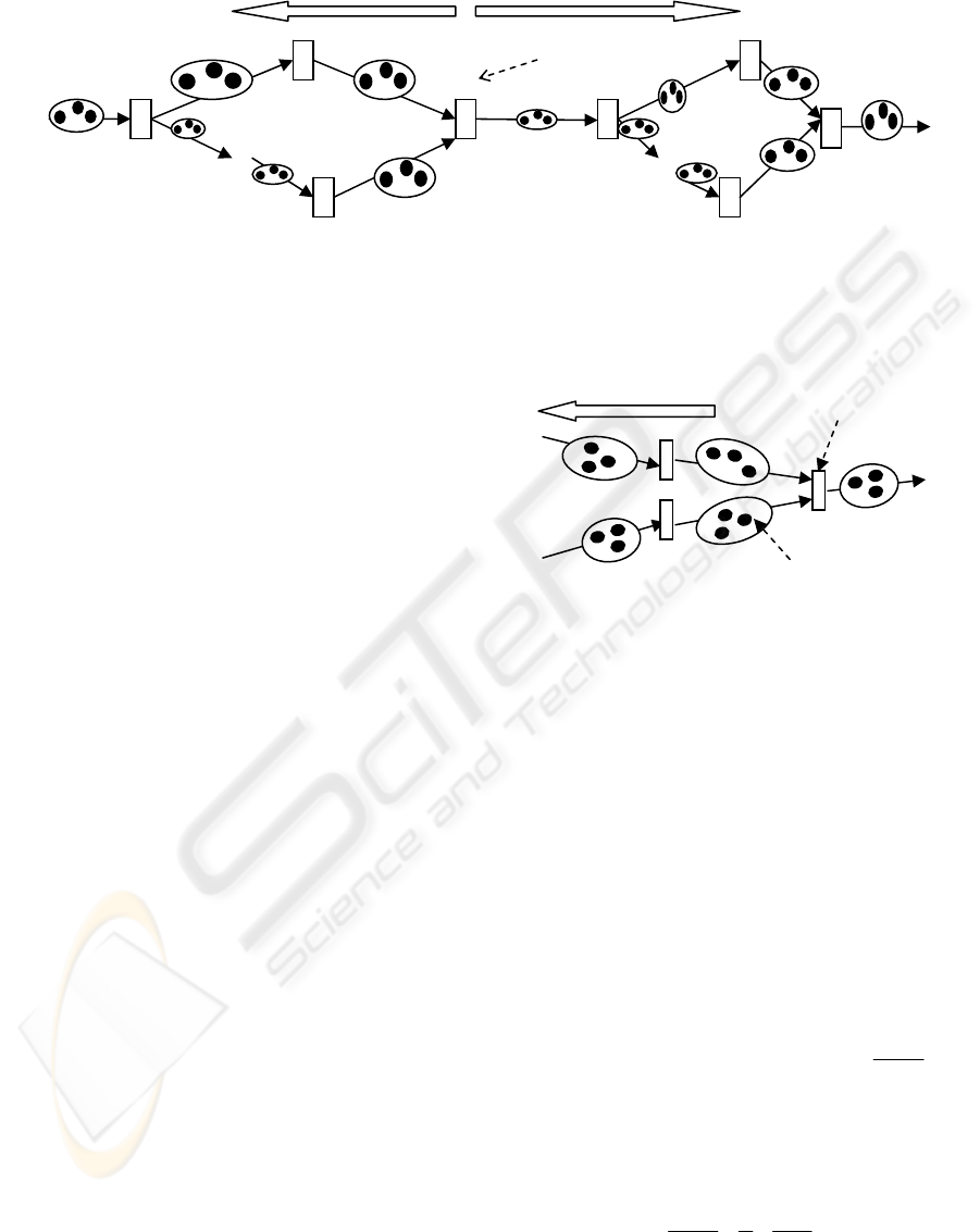
4.2 Analyzing Block Caused by a
Paused Transition
When a transition of a process model is paused
because of exception, the process will be blocked.
However, the block will not immediately be
propagated to the whole process because the size of
data buffer is not zero. The block propagation will
spend some time. In a long time, the final result is
that all the system is paused. For this situation, we
called it a Block Caused by a Paused Transition
pattern which is specified with Figure 4.2. For this
pattern, it is difficult to detect the problem from the
superficial phenomenon. And it is not easy to
simulate all the situations because there are a lot of
transitions and large number of paths. We must
provide theoretical analysis methods to handle this
pattern.
On the one hand, it will be useful to predicate the
situation, so that we can know how to control it. On
the other hand, some methods should be provided to
repair the paused system once this situation happens.
No matter we are preventing or repairing the
problem, computing the running speed of the
transitions is the foundation. Based on the running
speed, we will provide a method about how to
compute block propagation time.
Suppose a transition T
i+1
is paused, the block will be
propagated backward along a path. If a connection
from transition T
i
to T
i+1
exists, and the size of data
buffer between them is
i
C , and the effective speed
of transition T
i
is λ
i
V
, and the data input/output
structure of transition T
ˆ
i
is (N
i
)->(M
i
), then the
block propagation time from T
i
to T
i+1
is
ii
i
MV
C
ˆ
λ
.
Suppose T
1
->T
2
->…->T
n+1
is a path, and the T
n+1
is
the paused node, then the block propagation time
BPT(T
n+1
) from T
n+1
to T
1
can be computed using
the following formula:
BPT(T
n
) =
∑
=
n
i
ii
i
MV
C
1
ˆ
λ
=
∑
=
n
i
ii
i
MV
C
1
ˆ
1
λ
According to the above formula, we can have the
following conclusion:
Bottleneck
…
T
i
T
i+1
…
Figure 4.1 Input Data Flush Pattern
Reverse block
N
ormal
Figure 4.2: Block Caused by a Paused Node
p
aused node
b
lock
p
ro
p
a
g
ation direction
block here
A THEORETICAL PERFORMANCE ANALYSIS METHOD FOR BUSINESS PROCESS MODEL
79

1) If the value of
λ
is smaller, which indicates the
system is running at low performance level, a
process will spend longer time to be fully blocked
once a node is paused;
2) If the data buffer is the larger, the block
propagation time will be longer.
5 CONCLUSION
Detecting and improving business process
bottlenecks are critical for enterprise performance
improvement. This paper aims at a quantitative
analysis method for effectively and efficiently
detecting business process bottlenecks. A
computational model is proposed to abstract key
elements in business process model, including
transition, data, buffer and connections. Based on
this computational model, a Balance Equation
System is put forward to detect bottlenecks and the
solutions about how to improve the bottlenecks are
given. Furthermore, this approach was used to some
concrete applications. We classified the common
applications into some patterns, including large
number input data impact, block caused by a paused
node. Through using the theoretical analysis method,
these application patterns can be solved well.
Compared with traditional performance analysis
method, the theoretical analysis method in this paper
is easier and much more practical.
In a real business process, the performance of a
transition (the running speed of the transition) may
not be a constant, but depends on the resource
allocated to it. The more resource is allocated, the
better transition node performs we will have. From
the resource allocation point of view, a critical
resource can be allocated to multiple transitions.
Many applications run on the same server is the
typical example for this, in which applications are
transitions and the CPU power of the server is the
resource. How to best allocate the limited resource
to make the system achieve the highest performance
is an important topic for further study. In another
situation, the system performance may not be able to
meet the business requirements even though each
individual transition has reached its maximum
performance. This raises the problem of system
structure optimization. The challenge here is how to
change the system structure (the connection
structure of the model) to meet a specific high
requirements on performance. Changing the
bottleneck node into a parallel sub-structure can be a
example for this kind of structure optimization. The
analytical power of computational model will
provide a solid foundation for dealing with this kind
of problems.
REFERENCES
Christoph Roser, Masaru Nakano, Minoru Tanaka, 2003.
Comparison of Bottleneck Detection Methods for AGV
Systems. Proceedings of the 2003 Winter Simulation
Conference.
R. Blake and J. Breese, 1995. Automatic Bottleneck
Detection, Microsoft Technical Report MSR-TR-95-
10, Microsoft Corporation, October 1995.
Luthi, J., and Haring, 1997. G. Bottleneck Analysis for
Computer and Communication Systems with Workload
Variabilities & Uncertainties. In Proceedings of 2nd
International Symposium on Mathematical Modelling,
ed. I. Troch and F. Breitenecker, 525-534, 1997,
Vienna, Austria.
Lawrence, S. R., and Buss, A. H. 1995. Economic
Analysis of Production Bottlenecks. Mathematical
Problems in Engineering, 1(4): 341-369.
Christoph Roser, Masaru Nakano, 2001. Minoru Tanaka.
A Practical Bottleneck Detection Method. Proceedings
of the 2001 Winter Simulation Conference.
Donald Gross & Carl M. Harris, 1998. Fundamentals of
Queueing Theory, Third Edition Wiley-InterScience,
1998.
M.Ajmone Marsan, G.Balbo , and G.Conte, 1984. A Class
of Generalized Stochastic Petri Nets for the
Performance Analysis of Multiprocessor Systems,
ACM Trans. Computer Systems, vol. 2, no. 1, May
1984.
F.Baccelli and M.Canales, 1993. Parallel Simulation of
Stochastic Petri Nets Using Recursive Equations,
ACM Trans. Machines and Computer Systems, vol. 3,
pp. 20-41, 1993.
Salimifard K, Wright M, 2001. Petri net-based modelling
of workflow systems: an overview. European Journal
of Operational Research, 2001,134(3):664~676.
F.P.Kelly, R.J.Williams, 2004. Fluid model for a network
operating under a fair bandwidth-sharing policy. The
Annals of Applied Probability, 2004, Vol.14, No.3,
1055-1083.
Law, Averill M., and Kelton, David W, 1991. Simulation
Modelling & Analysis. McGraw Hill.
ICEIS 2005 - INFORMATION SYSTEMS ANALYSIS AND SPECIFICATION
80
