NONPARAMETRIC ANALYSIS OF SOFTWARE RELIABILITY

Revealing the Nature of Software Failure Dataseries

Andreas S. Andreou, Constantinos Leonidou

Department of Computer Science, University of Cyprus,

75 Kallipoleos Str., P.O.Box 20537, CY1678, Nicosia, Cyprus

Keywords: software failure, reliability, nonparametric analysis, antipersistence

Abstract: Software reliability is directly related to the number and time of occurrence of software failures. Thus, if we

were able to reveal and characterize the behavior of the evolution of actual software failures over time then

we could possibly build more accurate models for estimating and predicting software reliability. This paper

focuses on the study of the nature of empirical software failure data via a nonparametric statistical

framework. Six different time-series data expressing times between successive software failures were

investigated and a random behavior was detected with evidences favoring a pink noise explanation.

1 INTRODUCTION

System reliability is one of the major components

identified by the ISO9126 standard for assessing the

overall quality of software. More specifically,

software reliability can be evaluated on the

following factors:

• Maturity: Attributes of software that bear on

the frequency of failure by faults in the

software (

ISO/IEC 9126-1:2001)

• Fault tolerance: Attributes of software that

bear on its ability to maintain a specified level

of performance in cases of software faults or

of infringement of its specified interface

(

ISO/IEC 9126-1:2001)

• Crash frequency: The number of the system

crashes per unit of time

• Recoverability: Attributes of software that

bear on the capability to re-establish its level

of performance and recover the data directly

affected in case of a failure and on the time

and effort needed for it (

ISO/IEC 9126-1:2001)

The standard definition of reliability for software

is th

e probability of normal execution without failure

for a specified interval of time (Musa, 1999; Musa,

Iannino and Okumoto, 1987). Going a step further

we can state that reliability varies with execution

time and grows as faults underlying the occurred

failures are uncovered and corrected. Therefore,

measuring and studying quantities related to

software failure can lead to improved reliability and

customer satisfaction. There are four general ways

(quantities) to characterize (measure) failure

occurrences (Musa, 1999):

• Time of failure

• Time interval between failures

• Cumulative failures experienced up to a given

time t

• Failures experienced in a time interval t

The majority of recent research studies focus on

ftware reliability assessment or prediction using

the failure-related metrics mentioned above (e.g.

Patra, 2003; Tamura, Yamada and Kimura, 2003),

with very few exceptions that experiment with other

alternatives, like Fault Injection Theory (e.g. Voas

and Schneidewind, 2003), Genericity (Schobel-

Theuer, 2003), etc.

As Musa points out (Musa, 1999), the quantities

of fai

lure occurrences are random variables in the

sense that we do not know their values in a certain

time interval with certainty, or that we cannot

predict their exact values. This randomness, though,

does not imply any specific probability distribution

(e.g. uniform) and it is sourced on one hand by the

complex and unpredictable process of human errors

introduced when designing and programming, and

on the other by the unpredictable conditions of

program execution. In addition, the behavior of

software is affected by so many factors that a

deterministic model is impractical to catch.

138

S. Andreou A. and Leonidou C. (2005).

NONPARAMETRIC ANALYSIS OF SOFTWARE RELIABILITY Revealing the Nature of Software Failure Dataseries.

In Proceedings of the Seventh International Conference on Enterprise Information Systems, pages 138-145

DOI: 10.5220/0002517601380145

 SciTePress

The aim of this paper is to study the nature and

structure of software failure data using a set of

empirical software failure dataseries and a robust

nonparametric statistical method. The ReScaled

range (R/S) analysis, originated by Hurst (Hurst,

1956), looks deep in a time-series dataset and

provides strong evidences of either an underlying

deterministic structure, or a random behavior. In the

former case it can define the time pattern of the

deterministic behavior, while in the latter it reveals

the nature of randomness (i.e. the colour of noise).

The rest of the paper is organized as follows:

Section 2 outlines the basic concepts of the

nonparametric framework used to analyse the

available datasets. Section 3 describes briefly the six

software failure time-series data used and provides a

short statistical profile for the data involved. Section

4 concentrates on the empirical evidence that results

from the application of R/S analysis on the different

software projects failure data. In addition, this

section presents our attempt to investigate through

R/S Analysis the nature of software failure data

produced by two well-known and widely used

Software Reliability Growth Models, namely the

Musa Basic model and the logarithmic Poisson

Musa-Okumoto execution time model, and

compares results with those derived using the

empirically collected data. Finally, section 5 sums

up the empirical findings, draws the concluding

remarks and suggests future research steps.

2 THE R/S ANALYSIS

Technically, the origins of R/S analysis are related to

the “T to the one-half rule”, that is, to the formula

describing the Brownian motion (B.M.):

R = T

0.5

(1)

where R is the distance covered by a random particle

suspended in a fluid and T a time index. It is obvious

that (1) shows how R is scaling with time T in the

case of a random system, and this scaling is given by

the slope of the log(R) vs. log(T) plot, which is equal

to 0.5. Yet, when a system or a time series is not

independent (i.e. not a random B.M.), (1) cannot be

applied, so Hurst gave the following generalisation

of (1) which can be used in this case:

(R/S)

= c n

(2)

where (R/S)

is the ReScaled range statistic

measured over a time index n, c is a constant and H

the Hurst Exponent, which shows how the R/S

statistic is scaling with time.

The objective of the R/S method is to estimate

the Hurst exponent, which, as we shall see, can

characterise a time series. This can be done by

transforming (2) to:

log (R/S)

= log(c) + H log(n) (3)

and H can be estimated as the slope of the log/log

plot of (R/S)

vs. n.

Given a time series {X

: t=1,...,N}, the R/S

statistic can be defined as the range of cumulative

deviations from the mean of the series, rescaled by

the standard deviation. The analytical procedure to

estimate the (R/S)

values, as well as the Hurst

exponent by applying (3), is described in the

following steps :

Step 1: The time period spanned by the time series

of length N, is divided into m contiguous sub-periods

of length n such that mn = N. The elements in each

sub-period X

i,j

have two subscripts, the first (i=1,..,n)

to denote the number of elements in each sub-period

and the second (j=1,...,m) to denote the sub-period

index. For each sub-period j the R/S statistic is

calculated, as:

⎥

⎦

⎤

⎢

⎣

⎡

−−−=

⎟

⎠

⎞

⎜

⎝

⎛

∑∑

≤≤

−

jij

XXXXs

)(min)(max

(4)

where s

is the standard deviation for each sub-

period.

In (4), the k deviations from the mean of the sub-

period have zero mean; hence the last value of the

cumulative deviations for each sub-period will

always be zero. Due to this, the maximum value of

the cumulative deviations will always be greater or

equal to zero, while the minimum value will always

be less or equal to zero. Hence, the range value (the

bracketed term in (4)), will always be non-negative.

Normalizing (rescaling) the range is important since

it permits diverse phenomena and time periods to be

compared, which means that R/S analysis can

describe time series with no characteristic scale.

Step 2: The (R/S)

, which is the R/S statistic for time

length n, is given by the average of the (R/S)

values

for all the m contiguous sub-periods with length n,

as :

∑

⎟

⎠

⎞

⎜

⎝

⎛

⎟

⎠

⎞

⎜

⎝

⎛

(5)

Step 3: Equation (5) gives the R/S value, which

corresponds to a certain time interval of length n. In

order to apply equation (3), steps 1 and 2 are

repeated by increasing n to the next integer value,

until n = N/2, since, at least two sub-periods are

needed, to avoid bias.

From the above procedure it becomes obvious that

the time dimension is included in the R/S analysis by

examining whether the range of the cumulative

deviations depends on the length of time used for the

measurement. Once (5) is evaluated for different n

NONPARAMETRIC ANALYSIS OF SOFTWARE RELIABILITY: Revealing the Nature of Software Failure Dataseries

139

periods, the Hurst exponent can be estimated

through an ordinary least square regression from (3).

The Hurst exponent takes values from 0 to 1

(0≤H≤1). Gaussian random walks, or, more

generally, independent processes, give H = 0.5. If

0.5 ≤ H ≤1, positive dependence is indicated, and the

series is called persistent or trend reinforcing, and in

terms of equation (1), the system covers more

distance than a random one. In this case the series is

characterised by a long memory process with no

characteristic time scale. The lack of characteristic

time scale (scale invariance) and the existence of a

power law (the log/log plot), are the key

characteristics of a fractal series. If 0 ≤H ≤0.5,

negative dependence is indicated, yielding anti-

persistent or mean-reverting behavior

. In terms of

equation (1), the system covers less distance than a

random series, which means that it reverses itself

more frequently than a random process.

A Hurst exponent different from 0.5 may

characterise a series as fractal. However a fractal

series might be the output of different kinds of

systems. A “pure” Hurst process is a fractional

Brownian motion (Mandelbrot and Wallis, 1969),

also known as biased random walk or fractal noise

or coloured noise, that is, a random series the bias of

which can change abruptly but randomly in direction

or magnitude.

A problem, though, that must be dealt is the

sensitivity of R/S analysis to short-term dependence,

which can lead to unreliable results (Aydogan and

Booth, 1988; Booth and Koveos, 1983; Lo, 1991).

Peters (Peters, 1994) shows that Autoregressive

(AR), Moving Average (MA) and mixed ARMA

processes exhibit Hurst effects, but once short-term

memory is filtered out by an AR(1) specification,

these effects cease to exist. On the contrary, ARCH

and GARCH models do not exhibit long term

memory and persistence effects at all. Hence, a

series should be pre-filtered for short-term linear

dependence before applying the R/S analysis. In our

analysis, we use partial autocorrelograms and

Schwartz´s information criterion to indicate the best-

fit time series linear model to our data.

3 SOFTWARE FAILURE DATA

Before moving to applying R/S Analysis on the

available software failure datasets, let us examine

some basic features of the data: Six different

Only if the system under study is assumed to have a

stable mean

datasets were used in this paper, which were

collected throughout the mid 1970s by John Musa,

representing projects from a variety of applications

including real time command and control, word

processing, commercial, and military applications

(DFC, www.dacs.dtic.mil): Project 5 (831 total

samples), SS1B (375 total samples), SS3 (278 total

samples), SS1C (277 total samples), SS4 (196 total

samples) and SS2 (192 total samples).

R/S analysis can be applied only on a

transformation of the original data samples which

produces the so-called return series eliminating any

trend present. This transformation is the following:

⎟

⎠

⎞

⎜

⎝

⎛

−1

log

(6)

where S

and S

t-1

are the failure samples (more

specifically, the elapsed times form the previous

failure measured in seconds) at times (t) and (t-1)

respectively (discrete sample number) and r

is the

estimated return sample.

As mentioned in the previous section, in order to

remove the short-term memory all return series were

filtered with an AR(1) model. A short statistical

profile is depicted in Table 1, where one can easily

discern that the series under study present slight

differences from the normal distribution: Left

skewness is evident for all data series, while, as

regards kurtosis, Project 5 samples present

leptokurtosis with the rest series being less

concentrated around the mean compared to the

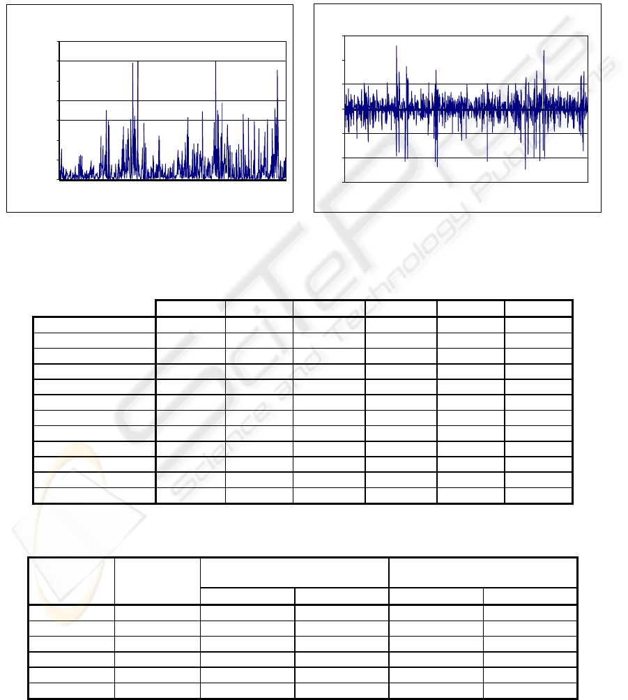
normal distribution. Figure 1 plots the data samples

belonging to Project 5, with the left figure showing

the evolution of failures according to the elapsed

time and the right figure presenting the de-trended

return series. The rest of the datasets present a

similar graphical representation, thus their figures

were omitted due to space limitations.

The statistical profile of the dataseries given

above suggests a general resemblance with the

normal (Gaussian random) distribution, but slight

differences were also observed. The main questions,

though, remain: What is the actual nature of this

data? Is there a random component in the behavior

of these series? The answers will be provided by

closely examining the results derived from the

application of R/S Analysis described in the next

section.

ICEIS 2005 - DATABASES AND INFORMATION SYSTEMS INTEGRATION

140

4 EMPIRICAL EVIDENCE

These Hurst exponent values indicate anti-

persistency, that is, all return series present negative

dependence or antipersistence, yielding a mean-

reverting behavior since the data fluctuate around a

reasonably stable mean (no trend or consistent

pattern of growth). In terms of equation (1), each of

the six systems covers less distance than a random

series, which means that it reverses itself more

frequently than a random process.

4.1 R/S Analysis Results on Software

Reliability Data Series

The results of R/S analysis on the six failure return

series are listed in Table 2. The Hurst exponent

estimated has a low value ranging from 0.27 (Project

5 dataset) to 0.37 (SS1C dataset).

AR(1)-filtered returns for the "Pro

ect 5" software

failure dataset

-6

-4

-2

1 61 121 181 241 301 361 421 481 541 601 661 721 781

sample

return

Time intervals between successive software

failures for the "Project 5" dataset

50000

100000

150000

200000

250000

300000

350000

1 61 121 181 241 301 361 421 481 541 601 661 721 781

failure number

seconds

(a) (b)

Figure 1: Project 5 sample series: (a) Time intervals between successive failures (b) AR(1)

Table 1: Statistical description of the six software failure returns series data (AR(1)-filtered samples)

Project 5 SS1B SS3 SS1C SS4 SS2

Sample size

829 373 276 275 194 191

Average

5.55E-18 2.97E-18 -1.20E-18 -5.85E-18 1.54E-17 3.95E-17

Median

0.024 0.073 0.075 0.084 0.121 -0.027

Variance

1.150 0.871 1.936 0.988 1.421 1.176

Standard deviation

1.072 0.933 1.391 0.993 1.192 1.084

Minimum

-4.963 -3.120 -5.056 -3.094 -4.127 -2.634

Maximum

5.165 2.879 3.470 4.786 2.832 3.268

Range

10.129 6.000 8.526 7.881 6.960 5.902

Lower quartile

-0.479 -0.536 -0.761 -0.473 -0.699 -0.671

Upper quartile

0.597 0.619 0.942 0.563 0.823 0.712

Skewness

-0.616 -0.263 -0.315 -0.034 -0.432 -0.131

Kurtosis

4.082 0.457 0.180 2.327 0.713 -0.019

Table 2: Hurst estimates and test of significance against two random alternatives for the AR(1)-filtered

returns series of the six different Musa’s software failure datasets

IID-null

Hypothesis

Gaussian-null

Hypothesis

Dataset

Hurst

Exponent

Mean Hurst Significance Mean Hurst Significance

Project5 0.27 0.56 0.1% 0.56 0.1%

SS1B 0.31 0.58 0.1% 0.58 0.1%

SS3 0.28 0.59 0.1% 0.60 0.1%

SS1C 0.37 0.59 0.1% 0.59 0.1%

SS4 0.33 0.60 0.1% 0.60 0.1%

SS2 0.33 0.60 0.1% 0.60 0.1%

NONPARAMETRIC ANALYSIS OF SOFTWARE RELIABILITY: Revealing the Nature of Software Failure Dataseries

141

A significant problem of R/S analysis is the

eva

lts obtained using the R/S

ana

m null, the H

est against the iid null, the same procedure is

tion of the R/S analysis results was

per

resembles the one observed for random, non-white

laws, which essentially is a function of

freq

b is the spectral component and H the

Hur t. T e can relate pi

to a

can conclude

tha

nalysis and Software

ystem

Havi ults thus far and the evidences

suggesting a pink noise explanation for the behavior

luation of the H exponent from a statistical point

of view. Specifically, we should be able to assess

whether an H value is statistically significant

compared to a random null, i.e. to the H exponent

exhibited by an independent random system. Peters

(1994) shows that under the Gaussian null, a

modification of a formula developed by Anis and

Lloyd (1976) allows for hypothesis testing by

computing E(R/S)

and E(H), the expected variance

of which will depend only on the total sample size

N, as Var(H)=1/N. However, if the null is still iid

randomness but not Gaussianity, the formal

hypothesis testing is not possible. To overcome this

problem we used bootstrapping (Efron, 1979) to

assess the statistical significance of the H exponents

of our series, against both the Gaussian and the iid

random null hypotheses.

The validity of the resu

lysis may be assessed as follows:

(A) To test against the Gaussian rando

exponent from 5000 random shuffles of a Gaussian

random surrogate, having the same length, mean and

variance with our return series is calculated and

compared to the test statistic i.e. the actual H

exponent of our series. Since the actual H statistic

was found to be lower than 0.5 and anti-persistence

is possible, the null can be formed as: H

: H = H

and the alternative is

: H < H

. In this case, the

significance level of the test is constructed as the

frequency with which the pseudostatistic H

smaller than or equal to the actual statistic and the

null is rejected if the significance level is smaller

than the conventional rejection levels of 1%, 2.5%

or 5%.

(B) To t

followed but this time we randomise the return

series tested to produce 5000 iid random samples

having the same length and distributional

characteristics as the original series. In this case,

rejection of the null means that the actual H

exponent calculated from the original series is

significantly smaller from the one calculated from an

iid random series. Hence, this is also a test for non-

iid-ness.

Valida

formed as described above, with both tests being

applied to the available dataseries. As Table 2

shows, both hypotheses are rejected since the

significance level of the test in both cases was lower

than 1%. This means that our Hurst estimates are

statistically significant against both the Gaussian and

the iid-null hypotheses suggesting an underlying

structure that deviates from normal distribution and

noise.

Fractional noise scales according to inverse

power

uency f, and follows the form f

-b

. This is a

typical characteristic of fractals, which have power

spectra that follows the inverse power law as a result

of the self-similar nature of the system (Peters,

1994). For white noise (Gaussian, random process)

b = 0, that is, the power spectra is not related to

frequency. There is no scaling law for white noise.

When white noise is integrated, then b = 2, the

power spectra for brown noise. If 0 < b < 2 we have

pink noise, while when b > 2 there is black noise.

Mandelbrot and Van Ness (Mandelbrot and Van

Ness, 1968) postulated, and recently Flandrin

(Flandrin, 1989) rigorously defined, the following

equation that relates fractional noises with the Hurst

exponent:

b = 2H + 1 (7)

where

st exponen herefore, w nk noise

ntipersistence: H < 0.50, 1 ≥ b > 2.

According to the foregoing notions, and based

on the results of the R/S analysis, we

t the six software failure data series are random in

nature, thus confirming the findings and supporting

the arguments of various researchers (Musa, 1999;

Musa and Iannino, 1990). Moving a step forward,

we may state that the main conclusion drawn is that

software failure empirical behavior resembles that of

pink noise.

4.2 R/S A

Reliability Growth Models S

Variables

ng in mind the res

of the empirical software failure data, we will

attempt to study the nature of the data produced by

known Software Reliability Growth Models

(SRGM) and compare results. Several studies (Dale,

1982; Ramamoorthy and Bastani, 1982; Farr, 1996;

Jones 1991) report the superiority of the Musa Basic

(MB) and the logarithmic Poisson Musa-Okumoto

(MO) execution time models (Musa, 1975; Musa

and Okumoto, 1984) over a variety of SRGM widely

applied to different actual projects and computer

programs. Therefore, we decided to use those two

models to produce new software failure time

samples and apply R/S analysis to investigate the

nature of the produced dataseries, and hence the type

ICEIS 2005 - DATABASES AND INFORMATION SYSTEMS INTEGRATION

142

of software failure behavior each model is capable to

capture. Let M(t) represent the number of failures of

the particular software package by time t, (t≥0). It is

clear that M(0)=0. M(t) cannot be easily calculated

because it corresponds to a physical quantity and can

only be measured as the software is tested. Software

Reliability Growth Models are trying to model the

behavior of M(t) with the statistical function µ(t).

The mean value function µ(t) of a SRGM represents

the number of failures expected to occur up to time

moment t, (t≥0):

Ntct )()( =

(8)

where c(t) is the time variant test coverag

func N is the number

hav

tion and of faults expected to

e been exposed at full coverage. This is

distinguished from the expected number of faults to

be detected after infinite testing time, perfect testing

and fault detection coverage, which can be denoted

. Equations (9) and (10) describe the test

coverage function for the MB and MO models

respectively:

MB :

fKBt

etc

−

−=1)(

(9)

MO :

)1ln()( ttc

(10)

where φ is e s the so-the failure rate p r fault, K i

call sure ratio, B is a fault r

fac

ed fault expo eduction

tor and f can be calculated as the average object

instruction execution rate of the computer r, divided

by the number of source code instructions of the

application under testing I

, times the average

number of object instructions per source code

instruction, Q

(Musa, 1999):

f =

(11)

Both M(t) q nc he form and µ(t) are se ue es of t

0,1,2, … with M(0)=0 and µ(0)=0. Assuming that as

ime t as t app

positive variable i, (i=0,1,2...). Thus, we

hav

Su g c(t

) in (9) and (10) and solving for t

approaches infinity µ(t) becomes a good

approximation of M(t) (the number of failures that

has been realized up to time t) we will have µ(t)

taking by definition integer positive values (since

µ(t) corresponds to the expected number of failures

experienced by time t; hence

[]

K,2,1,0)( ∈t

). Both

SRGMs (MB and MO) converge to the number of

failures being realized up to t roaches

infinity is generally acceptable. Therefore, our

assumption that M(t) will be approached by µ(t) as t

approaches infinity. But µ(t), which characterizes a

SRGM, is given as a model property, thus we should

try to reverse engineer the process of failure

occurrence and artificially reproduce the “ failure

occurrences”. The failure reproduction process is as

follows:

First we replace µ(t) in equation (8) with an

integer

i=c(t

)N (12)

bstitutin

hav

MB:

⎟

⎞

⎜

⎛

−−=⇔−=

−

tNei

fKBt

1ln

)1(

(13)

⎠⎝

NfKB

MO:

⎟

⎠

⎞

⎜

⎝

⎛

−=⇔+= 1

)1ln(

etNti

me variable t

represents discrete fa

moments, i.e. the time elapsed from the start of this

pro

(14)

ilure time

cess (t

for i=0) until the occurrence of the i

failure (t

for i=1, t

for i=2 etc.).

Consequently we can calculate times between

successive failures as:

escribed above, we

duc artific es d ta via e

failure dataseries were thus

5 CONCLUSIONS – DISCUSSION

The nature of empirical software reliability time

series data was investigated in this paper using a

∆t

= t

- t

i-1

. (15)

Following the analysis d

repro ed ial failure tim a quations

to 15, for which we used the following parameter

values suggested by Musa (1975, 1999) and the

Defense Software Collaboration (DFC,

www.dacs.dtic.mil):

φ = 7.8 E-8, f = 7.4 E-8, K = 4.2 E-7, B= 0.955

Two new software

enerated, with their size being equal to that of

Project 5 (829 samples). R/S analysis was then

applied on the AR(1)-filtered returns of the

artificially reproduced series. The Hurst exponent

estimations indicate that the MB-based reproduced

series exhibit long-memory or persistent effects

(H=0.9), while the corresponding MO-based sample

data is characterized as antipersistent (H=0.2). These

findings are very interesting considering the fact that

they suggest a strong diversification between two

models that are both used as software reliability

growth estimators, and hence as software failure

predictors. The similar antipersistent

characterization of the six software failure dataseries

under study and the MO-based generated data is also

consistent with the findings of other researchers who

report the superiority of the MO model in actual

software projects. It is therefore natural that this

model proved to be more successful compared to the

rest of the SRGMs simply because its underlying

modeling nature is similar to the behavior observed

with actual empirical data.

NONPARAMETRIC ANALYSIS OF SOFTWARE RELIABILITY: Revealing the Nature of Software Failure Dataseries

143

robust nonparametric statistical framework called

ReScaled range (R/S) analysis. This type of analysis

ing process should play a central role in the

pla

ast five years. We are trying to

bui

is able to detect the presence (or absence) of long-

term dependence, thus characterizing the system

under study as persistent / deterministic (or mean-

reverting / antipersistent).

The results of the R/S analysis on six different

software failure dataseries suggested a random

explanation, revealing strong antipersistent behavior.

The validity of these results was tested against the

ussian and iid-null hypotheses and both

alternatives were rejected with highly significant

statistical values. Our findings are consistent with

other reports in the international literature that

comment on the random nature of software failures

in terms of number and time of occurrence. Going a

step further and relating the values of the Hurst

exponent estimated via the R/S analysis with colored

noise, we concluded that the six series examined are

better described by a pink noise structure.

Two well known and successful software

reliability growth models, namely the Musa Basic

(MB) and the Musa-Okumoto (MO) logarithmic

model, were used to reproduce sample series of

tim

es between failures. The new series were also

tested with R/S analysis and found to be long-term

dependent in the case of the MB data and

antipersistent in the case of the MO series. The latter

finding justifies the superiority of the MO model

over a variety of other SRGM tested on a number of

actual projects: The MO model is ruled by the same

structure as the empirical software failure data (i.e.

mean reverting), thus it can capture the actual

behavior of software failures better.

The framework for statistical characterization of

empirical software failure data proposed by the

present work can assist towards the identification of

possible weaknesses in the assumptions of SRGMs

and

suggest the most suitable and accurate model to

be used for controlling the reliability level of the

software product under development.

One thing that remains to investigate, and this

will be the focus of our future work, is the high

value of the Hurst exponent for the MB series.

Chaotic systems have also Hurst exponents H > 0.5,

and

in chaotic terms long memory effects

correspond to sensitive dependence on initial

conditions. Actually, the latter property combined

with fractality characterises chaotic systems. Pure

chaotic processes have Hurst exponents close to 1.

Our future research will concentrate on employing

R/S analysis to detect the existence of cycles (i.e.

repeating patterns) in the MB series and will attempt

to characterise it in terms of periodicity: Cycles

detected can be periodic or non-periodic in the sense

that the system has no absolute frequency. Non-

periodic cycles can be further divided to statistical

cycles and chaotic cycles. Fractal noises exhibit

statistical cycles, i.e. cycles with no average cycle

length.

Software Reliability is cited by the majority of

users as the most important feature of software

products. Hence, the software reliability

engineer

nning and control of software development

activities (Musa, 1999) to ensure that product

reliability meets user needs, to reduce product costs

and to improve customer satisfaction. In this context,

it is quite important to record and study the time of

fault occurrences, their nature and the time spent on

correction, throughout the design and

implementation phases, as well as during testing

activities. This data can prove very useful when

trying to model the reliability behavior of the

software product being developed and it can also

play a central role to the empirical verification of

Software Reliability Growth Models (SRGMs).

With such data available it is easier to select suitable

reliability models for estimating the time at which

the software product will have reached a desirable

level of reliability, and/or to devise methods to

decrease that time. As we mentioned before, the

datasets used in this study were gathered by John

Musa around mid seventies. Although the datasets

are quite old, we believe that their analysis is a good

starting point for studying the behavior of software

failure occurrences.

Currently we are making efforts towards

gathering synchronous failure data, that is, data from

systems that have been developed and are in

operation during the l

ld a database with failure data from various

modern application domains and operating systems.

In our days, where most computer applications and

operating systems are multitasking and/or

distributed, it is very interesting to elaborate on how

to gather accurate failure data. This problem, the

definition of the right metrics to assess software

reliability, has a particular interest due to the fact

that software products nowadays include some new

and unique characteristics, such as distribute

computing, mobility and web accessibility /

immediacy. Once this reliability data gathering is

accomplished, we will be able to compare the

characteristics of modern reliability data with those

of the datasets developed by Musa in the 70ies, and

investigate whether the random nature of software

failure occurrences revealed by the R/S analysis

ICEIS 2005 - DATABASES AND INFORMATION SYSTEMS INTEGRATION

144

holds true for modern software systems as well.

Furthermore, we will attempt to investigate whether

there is a relationship between the datasets used and

the results obtained, i.e. whether certain application

domains are more error prone than others.

REFERENCES

Anis, A.A. and Lloyd E.H., 1976. The Expected Value of

endent

iometrica 63, pp. 155-164.

Aydogan, K. and Booth, G., 1988. Are there long cycles in

Bo ment

Da ware Reliability Evaluation Methods,

the Adjusted Rescaled Hurst Range of Indep

Normal Summands. B

common stock returns? Southern Economic Journal

55, pp. 141-149.

oth, G.G. and Koveos, P.E., 1983. Employ

fluctuations: an R/S analysis. Journal of Regional

Science 23, pp. 19-31.

le, C.J., 1982. Soft

Report ST26750, British Aerospace.

fense Software Collaboration,

http://

www.dacs.dtic.mil/techs/baselines/reliability. html

Efron, B., 1979. Bootstrap methods: Another look at the

jack-knife. The Annals of Statistics 7,

pp. 1-26.

ility

Fla ctional

Hu in

Inte rganization for Standardization, 1991.

ents with fractional Gaussian noises. Part 1, 2,

Ma Fractional

Mu tware Reliability. In

Mu re Reliability and its

Musa, J.D., Iannino, A., Okumoto, K., 1987. Software

national Conference on

Pat

ftware Reliability

Pet

ering 8(4), pp. 354-370.

on Software

Tam

networks for distributed development

IEEE

Farr, W., 1996. Software Reliability Modeling Survey. In

M. Lyu (ed.) Handbook of Software Reliab

Engineering, McGraw-Hill, New York, pp. 71-117.

ndrin, P., 1989. On the Spectrum of Fra

Brownian Motions, IEEE Transactions on Information

Theory 35.

rst, H.E, 1956. Methods of using long-term storage

reservoirs. Proceedings of the Institute of Civil

Engineers 1, pp. 519-543.

rnational O

ISO/IEC 9126 - Information Technology, Software

Product Evaluation, Quality, Characteristics and

Guidelines for their Use.

Jones, W.D., 1991. Reliability Models for Very Large

Software Systems in Industry, 2

International

Symposium on Software Reliability Engineering, pp.

35-42.

Lo, A.W., 1991. Long term memory in stock market

prices. Econometrica 59, pp. 1279-1313.

ndelbrot, B. and Wallis, J., 1969. Computer

experim

3. Water Resources Research 5.

ndelbrot, B. and van Ness, J.W., 1968.

Brownian Motions, Fractional Noises and

Applications, SIAM Review 10.

sa, J.D., Iannino, A., 1990. Sof

Marshall Yvotis (ed.) Advances in Computers 30, pp.

85-170, Academic Press, San Diego.

sa, J.D., 1975. A Theory of Softwa

Application, IEEE Trans. Software Eng. 1(3), pp. 312-

327.

Musa, J., 1999. Software Reliability Engineering,

McGraw-Hill, New York.

Reliability - Measurement, Prediction, Application,

McGraw-Hill, New York.

Musa, J.D., Okumoto, K., 1984. A Logarithmic Poisson

Execution Time model for Software Reliability

Measurement, 7

Inter

Software Engineering, pp. 230-238.

ra, S., 2003. A neural network approach for long-term

software MTTF prediction. In Fast abstracts of the 14

IEEE International Symposium on So

Engineering (ISSRE2003), Chillarege Press.

ers, E., 1994. Fractal market analysis: applying chaos

theory to investment and economics. New York: John

Wiley & Sons.

Ramamoorthy, C.V., Bastani, F.B., 1982. Software

Reliability – Status and Perspectives, IEEE Trans. On

Software Engine

Schobel-Theurer, T., 2003. Increasing software reliability

through the use of Genericity. In Fast abstracts of the

IEEE International Symposium

Reliability Engineering (ISSRE2003), Chillarege

Press.

ura, Y., Yamada, S. and Kimura, M., 2003. A

software reliability assessment method based on

neural

environment. Electronics and Communications in

Japan, Part 3, Vol. 86, No. 11, pp. 1236-1243.

as, J. and Schneidewind, N., 2003. Marrying software

Fault Injection Technology with Software Reliability

Growth Models. In Fast abstracts of the 14

International Symposium on Software Reliability

Engineering (ISSRE2003), Chillarege Press.

NONPARAMETRIC ANALYSIS OF SOFTWARE RELIABILITY: Revealing the Nature of Software Failure Dataseries

145