
AN APPLICATION OF NON-LINEAR PROGRAMMING TO
TRAIN RECURRENT NEURAL NETWORKS IN TIME SERIES
PREDICTION PROBLEMS
M.P. Cuéllar, M. Delgado, M.C. Pegalajar
Department of Computer Science and Artificial Intelligence. E.T.S. Ingeniería Informática. Univerity of Granada, C/. Pdta
Daniel Saucedo Aranda, s.n.. Granada (Spain, Europe)
Keywords: Non-Linear Programming, Recurrent Neural Networks, Time Series Prediction
Abstract: Artificial Neural Networks are bioinspired mathematical models that have been widely used to solve many
complex problems. However, the training of a Neural Network is a difficult task since the traditional
training algorithms may get trapped into local solutions easily. This problem is greater in Recurrent Neural
Networks, where the traditional training algorithms sometimes provide unsuitable solutions. Some
evolutionary techniques have also been used to improve the training stage, and to overcome such local
solutions, but they have the disadvantage that the time taken to train the network is high. The objective of
this work is to show that the use of some non-linear programming techniques is a good choice to train a
Neural Network, since they may provide suitable solutions quickly. In the experimental section, we apply
the models proposed to train an Elman Recurrent Neural Network in real-life Time Series Prediction
problems.
1 INTRODUCTION
Artificial Neural Networks are bioinspired
mathematical models that have been widely used to
solve many complex problems, difficult to model
because of their non-linearity, lack of information,
or excessive difficulty. The most common neural
network models used to solve these problems have
mainly been feedforward networks (Haykin, 1999).
There are many training algorithms for this kind of
network and most are based on error propagation
methods: for instance, backpropagation algorithms
and similar ones. However, the disadvantage of
these algorithms is that the search for the best
solution is frequently trapped in a local optimum,
therefore making it difficult for the network to work
well.
In the case of Recurrent Neural Networks (D.P.
Mandic et al., 2001), there are not as many training
algorithms as for feedforward ones. These
algorithms (M. Hüsken et al., 2003; R.J. Williams et
al., 1989-1990) also share the same disadvantage as
those used to train feedforward networks in that they
get trapped in local optimal solutions very easily. In
fact, This problem is greater in recurrent neural
networks. Some evolutionary techniques have been
proposed as a good choice to train these kind of
networks (Blanco et al., 2001; M.P. Cuéllar et al.,
2004), because they can overcome the local optimal
solutions, but they have the drawback that the
training stage takes too much time.
In this work, we propose some non-linear
programming algorithms to train Recurrent Neural
Networks. These algorithms are the BFGS (C. Zhu
et al., 1997; R.H. Byrd et al., 1995) and the
Levenberg-Marquardt minimization methods. Both
algorithms are related to the Gauss-Newton method,
but the implementations used in this work may be
used to solve different kind of problems, as we will
show in section 3.
Related to Neural Network training, the BFGS
method has been used to train feedforward networks,
being hybridized with the evolutionary Scatter
Search algorithm (R. Martí et al., 2002), in order to
improve the solutions during the evolutionary
process, obtaining suitable results in function
approximation problems. On the other hand, the
Levenberg-Marquardt (LM) (D.W. Marquardt, 1963;
J.J More, 1977) method is a widely known algorithm
used to optimize Radial Basis Function Networks
(R. Zemomi, 2003). Some implementations have
adapted the LM algorithm to train feedforward
35
P. Cuéllar M., Delgado M. and C. Pegalajar M. (2005).
AN APPLICATION OF NON-LINEAR PROGRAMMING TO TRAIN RECURRENT NEURAL NETWORKS IN TIME SERIES PREDICTION PROBLEMS.
In Proceedings of the Seventh International Conference on Enterprise Information Systems, pages 35-42
DOI: 10.5220/0002515800350042
Copyright
c
SciTePress
networks (M.T. Hagan et al., 1994). Other
applications of both algorithms are ralated to solve
minimization problems.
In this work, we use the models proposed to train
an Elman Recurrent Neural Network (ERNN) (D.P.
Mandic et al., 2001) in real-life Time Series
prediction problems. The reasons to choose an
ERNN model are mainly related to the problem to
solve:
Time Series are, basically, a data chaining,
indexed in time. Such data chaining often has some
temporal properties, in the sense that the value of the
Time Series at the current time depends on some
unknown past values. The objective of Time Series
Prediction is to model the Time Series, and then to
predict the future values with minimum error. Many
approaches have been used to model a Time Series,
and to the date, it is still a great problem. Traditional
techniques, basically statistical methods, are very
limited, since the models used are mainly linear
regressions, and the temporal properties of the time
series are often non-linear ones. In recent works,
there are many approaches to model a Time Series
with non-linear models, and Neural Networks play a
great role in this field. The use of RBF Networks is
very common in Time Series Prediction (R. Zemomi
et al., 2003), but they have the disadvantage that the
analysis of the temporal properties must be done
manually, therefore increasing the number of
experiments. Recurrent Neural Networks is a
suitable approach to model a Time Series, since the
recurrence allows the network to learn the temporal
properties that the input data have, and the analysis
of the temporal properties is done automatically.
Considering some models of Recurrent Networks,
the ERNN has obtained the best experimental results
in our work.
This work is structured as follows: Section 2
introduces the Elman Recurrent Neural Neural
Network. In section 3, the non-linear programming
algorithms proposed are exposed. Section 4 shows
the experimenta results obtained. Finally, section 5
discusses the conclusions obtained.
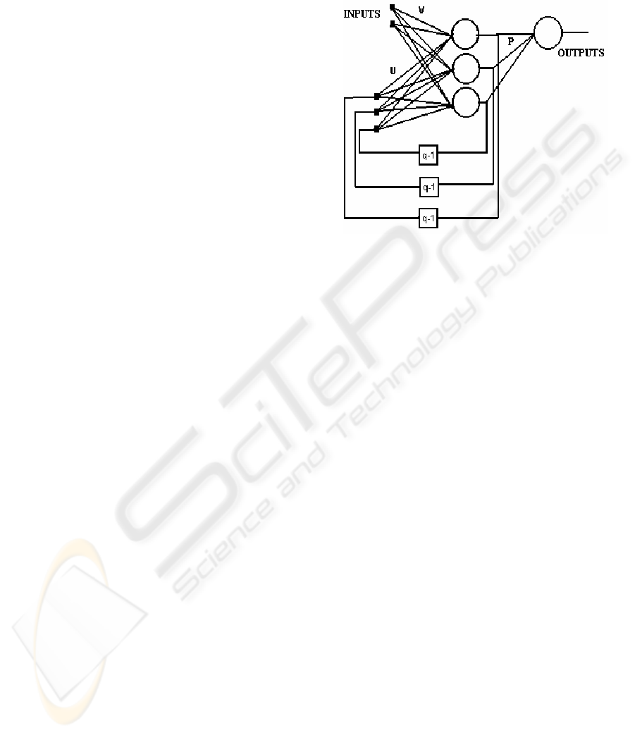
2 ELMAN RECURRENT NEURAL
NETWORKS
An Elman recurrent neural network has three neuron
layers: one is used for the input data, another is the
hidden neuron layer, and the other is the output
neuron layer. The network also has an additional
neuron layer, called the state neuron layer. There are
as many neurons in the state neuron layer as there
are in the hidden layer. Recurrence is carried out
from the hidden neurons to the state neurons so that
the output of a hidden neuron at time t is also input
to all hidden neurons at time t+1. This idea is
illustrated in Figure 1.
Figure 1 shows an example of an Elman recurrent
neural network with two inputs, one output, and
three hidden neurons. Therefore, the state neuron
layer also has three neurons, corresponding to the
values of the three hidden nodes at the previous
time. The equations of the network dynamics are:
(1)
(2)
(3)
(4)
where:
• Y
B
k
B(t) is the output of neuron k in the output
layer, at time t.
• Netout
B
k
B(t) is the output of neuron k in the
output layer, when the activation function has
not yet been applied.
• Neth
B
k
B(t) is the output of neuron k in the hidden
layer, when the activation function has not yet
been applied.
• S
B
k
B(t) is the output of neuron k in the hidden
layer.
• H is the number of neurons in the hidden layer.
• I is the number of neurons in the input layer.
• S
B
k
B(t-1) is the state value, corresponding to the
state neuron k, at time t.
)G(netout(t)Y
kk
=
∑∑
==
+−=
H
1h
I
1i
ijihjhh
(t)XV1)(tSU(t)neth
(t))f(neth(t)S
jj
=
∑
=
=
H
0j
jkjk
(t)SP(t)netout
Figure 1: Example of an Elman recurrent neural
network with two intputs, three hidden neurons, and
one output
ICEIS 2005 - ARTIFICIAL INTELLIGENCE AND DECISION SUPPORT SYSTEMS
36

• F(·) is the activation function of the neurons in
the hidden layer.
• G(·) is the activation function of the neurons in
the output layer.
• V
B
ij
B is the weight of connection from neuron j in
the input layer to neuron i in the hidden layer.
• U
B
ij
B is the weight of connection from neuron j in
the state layer to neuron i in the hidden layer.
• P
B
ij
B is the weight of connection from neuron j in
the hidden layer to neuron i in the output layer.
• X
B
i
B(t) is the network input i at time t.
The traditional gradient-based training algorithm
used to train this kind of network is the
Backpropagation Through Time (BPTT) algorithm.
The main drawback of this algorithm, as shown in
section 1, is that the method gets trapped into local
optimal solutions very easily.
In the following section, the non-linear
programming algorithms proposed in this work, and
its application to Recurrent Neural Network training,
are introduced.
3 NON-LINEAR PROGRAMMING
ALGORITHMS
Before to explain the BFGS and the LM algorithms,
an introduction to non-linear programming is shown.
A non-linear program is a problem that can be
considered as a minimization task with the following
structure:
(5)
The function F is called objective function, x is a
vector of n variables to be optimized. The functions
g
B
i
B and hB
j
B are called constraint equations. The
constraint equations remark some conditions that
must be fulfilled for a set of variables in x. If the
value m=0, then there are no conditions or
dependencies in the variables in x, and the problem
is called unconstrained.
There are many reasons to choose the BFGS and
the LM algorithms in this work. These are:
- They have been applied to optimize
feedforward neural networks, obtaining good
results. Therefore, it may be interesting to
apply them to train recurrent networks,
where the training stage is more difficult.
- The versions of the algorithms implemented
in this work may be applied to problems with
different characteristics, as shown below.
Depending on the problem to solve, it may be
classified, considering the number of training data,
into underdetermined, determined, and
overdetermined problems. A problem is
underdetermined when there are less training
examples than variables to optimize; it is determined
when there are as many training examples as
variables to optimize, and overdetermined when
there are more training examples than variables to
optimize. The determined problems are not very
common, so that in this work we only consider the
underdetermined and the overdetermined problems.
Furthermore, in some applications of Recurrent
Neural Networks, it may be interesting to keep the
weight values belonging not to ℜ, but to a valid
interval in ℜ. An example of this situation is when
the neural network must be implemented in
hardware, and the number of bits to represent a
weight is fixed. We can see this situation as a
constrained situation, so that we can also classify the
problems into constrained and unconstrained
problems.
Attending to the previous classifications, the
BFGS and the LM algorithms proposed in this work
may be applied to a concrete kind of problems, as
shown in tables 1 and 2.
Unconstrain
ed problems
Constrained
problems
Underdetermined
problems
NO NO
Overdetermined
problems
YES NO
Table 2: Problems solved by BFGS
Unconstrain
ed problems
Constrained
problems
Underdetermined
problems
YES YES
Overdetermined
problems
YES YES
As we can see, the applications of BFGS also
include the problems solved by LM. However, in the
experimental section, we show that the solutions
provided by LM are much better than the ones
1
1
1j
1i
n
mm
0m
1,..mmj0,)x(h
1..mi0,)x(g
:tosubject
),xF(minimize
≥
≥
+=≥
==
ℜ∈x
Table 1: Problems solved by LM
AN APPLICATION OF NON-LINEAR PROGRAMMING TO TRAIN RECURRENT NEURAL NETWORKS IN TIME
SERIES PREDICTION PROBLEMS
37

provided by BFGS for overdetermined
unconstrained problems.
Below, subsections 3.1 and 3.2 explain the BFGS
and the LM algorithms, and their application to
Recurrent Neural Network training.
3.1 The BFGS algorithm
The BFGS algorithm was firstly proposed in 1970
by Broyden, Fletcher, Goldfarb and Shanno. Since
then, several approaches to improve the algorithm,
and also to apply it to a wider set of problems, have
been proposed. In this work, we use an adaptation of
this algorithm, called limited-memory bound-
constrained/unconstrained BFGS algorithm (L-
BFGS-B) (R. H. Byrd et al., 1995). The L-BFGS-B
algorithm solves a problem that is considered as
shown in equation 5, where the constraint equations
are basically bound constraints, it is said:
h
B
j
B(x)= lB
j
B ≤xB
j
B ≤uB
j
B, j=1..n
where l
B
j
B and uB
j
B are the lower and upper bounds for
the variable to optimize x
B
j
B, respectively. The main
scheme of the algorithm is shown below:
0. At the beginning, a solution x
B
k
B, k=0, and the
corresponding gradient for function F must
be provided as input data.
1. If the search has converged, stop.
2. Find an initial local solution, by mean of
calculating the Cauchy point.
3. Compute a search direction, called d
B
k
B.
4. Perform a line search along d
B
k
B, subject to the
bound constraints, in order to compute the
step length λ
B
k
B, and set xB
k+1
B=xB
k
B+λB
k
B dB
k
B.
5. Compute
∇
F(xB
k+1
B)
6. Update the limited-memory matrices, if
necessary.
7. Set k= k+1, and go to Step 1.
Firstly, the algorithm computes an initial solution
and a search direction, d
B
k
B. Then, the solution is
modified according to d
B
k
B. The algorithm also apply a
Quasi-Newton algorithm to approximate the Hessian
matrix. In (C. Zhu et al., 1997; R.H. Byrd et al.,
1995), you can find an in-depth explanation about
this algorithm.
Now, the use of the L-BFGS-B algorithm to train
an ERNN is explained. Firstly, an ERNN is
considered as a non-linear program (equation 5).
After that, we show how to calculate the gradient of
the variables to be optimized.
When training a neural network, the objective is
to minimize the output error. One of the most
common procedures used to do this, is to minimize
the Mean Square Error (MSE) between the network
output, and the desired output for the network. In the
case of recurrent neural networks, the MSE must be
minimized across the time, as equation 6 shows.
(6)
where w is a vector containing the network weights,
T is the number of training samples in the time, O is
the number of network outputs, d
B
o
B(t) is the desired
output for neuron o at time t, and Y
B
o
B(t) is the
network output provided by neuron o at time t (see
equation 4). According to the notation introduced in
Section 2, the vector w is structured as follows:
Thus, equation 5 may be rewritten as follows:
(7)
The area in brackets is optional, and it contains the
bound constraints in constrained problems.
The gradient value for a variable w
B
r
B, denoted qB
r
B,
that must be provided to the algorithm, is calculated
in the following way:
Now, a vector Q, with the gradient values for the
variables in vector w, may be defined as follows:
∑
∑
=
=
−=
=
O
1o
2
oo
T
1t
(t))d(t)(Yt),wSE(
t),wSE(
T
1
)wMSE(
})w{MSE(min
)...P..PP..PP...U...U
..U..UU...VV..VV(Vw
OH2H211H11HH2H
211H11HI211I1211
=
⎥
⎦
⎤
⎢
⎣
⎡
=≤≤
ℜ∈
∑
=
njuwl
w
jjj
..1,
:tosubject
},t),wSE(
T
1
{minimize
n
T
1t
r
r
w
)wMSE(
q
∂
∂
=
1..nr),(qQ
r
==
ICEIS 2005 - ARTIFICIAL INTELLIGENCE AND DECISION SUPPORT SYSTEMS
38

The gradient value for each variable in w, using
the notation from Section 2, is calculated below:
Where 1≤i≤I, 1≤j≤H, 1≤o≤O. Thus, the gradient
vector Q may be rewritten, following the same order
defined for the vector w, as follows:
You can find a Fortran free source code of the L-
BFGS-B algorithm in the web site
http://www.ece.northwestern.edu/~nocedal/lbfgsb.ht
ml. In this work, we have translated it to C language,
and also to adapt such source code in order to train
ERNN.
3.2 The LM algorithm
The basic LM algorithm was proposed by D.W.
Marquardt in (D.W. Marquardt, 1963). Since then,
there are many approaches to solve a non-linear
program using the LM algorithm.
The algorithm tries to fit n parameters x
B
1
B...xB
n
B, in a
non-linear problem. The initial assumption is that,
sufficiently closed to the minimum of the function F
to be minimized, F may be approximated by a
quadratic form:
where h is a n-dimensional vector, and H is the
Hessian matrix. If the approximation is good, then
the optimal values for w may be calculated.
Otherwise, the algorithm iterates using the steepest
descent method (S. Haykin, 1999) in order to
improve the current solution. The main scheme of
the algorithm is structured as follows:
0. At the beginning, a solution x
P
k
P
, k=0, and a
step-length parameter λ, must be provided as
input data.
1. Compute F(x
P
k
P
)
2. Update the Hessian matrix, and calculate
δ
xP
k
P
3. Compute F(x
P
k
P
+
δ
xP
k
P
).
4. If (F(x
P
k
P
+
δ
xP
k
P
)
≥
F(xP
k
P
)), increase λ by a factor
of 10
5. If (F(x
P
k
P
+
δ
xP
k
P
) < F(xP
k
P
)), then
5.1. decrease λ by a factor of 10
5.2. set x
P
k+1
P
= xP
k
P
+
δ
x
6. Set k= k+1
7. If the algorithm has converged, stop.
Otherwise, go to step 1.
The implementation used in this work solves an
overdetermined set of non-linear equations by mean
of a modification of the LM algorithm. You can find
a good explanation of the implementation of this
algorithm in (J.J. More, 1977).
Now, the training process for ERNN, using the
LM algorithm, is explained. The training of an
Elman Recurrent Neural Network may be
considered as the fitting of set of m non-linear
equations, being m the number of training samples:
(8)
Considering equation 8, m=T·O, where T is
the number of training samples, and O is the number
of network outputs; d
B
o
B(t) is the desired output for
neuron o at time t, and Y
B
o
B(t) is the network output
provided by neuron o at time t.
Being considered an Elman Recurrent Neural
Network as a set of m equations as shown in (8), the
LM algorithm minimizes the sum of the squares for
such m equations. Thus, equation 5 may be rewritten
as follows:
(9)
Thus, equation 9 shows the function to be
minimized, and the LM algorithm may be applied
directly.
There is an important advantage in the LM
algorithm, being compared with BFGS. To explain
it, we must take a look at equations 7 and 9. In (7),
the function to minimize is the MSE across the time.
Please note that the minimization is carried out for
the sum of the errors in output values. On the other
hand, equation (9) minimizes the errors for each
⎩
⎨
⎧
=
=
−=
1..Oo
1..Tt
(t);d(t)Yt),w(F
ooo
}t)),w((F{min
T
1t
O
1o
2
o
∑∑
==
xHx
2
1
xhγF +−≈
∑
∑
∑
∑
=
=
=
=
−=
=
∂
∂
−=
∂
∂
−=
∂
∂
O
1o
ooojjj
T
1t
ji
ji
T
1t
jk
jk
T
1t
joo
oj
(t))d(t)(YP(t))(nethf'
T
2
(t))δ(S
(t)))(S(t)(X
V
t),wMSE(
(t)))(S1)(tS
U
t),wMSE(
(t)(t))Sd(t)(Y
T
2
P
t),wMSE(
δ
δ
)
dP
t),wMSE(
..
dU
t),wMSE(
..
dV
t),wMSE(
(Q
okjkji
∂∂∂
=
AN APPLICATION OF NON-LINEAR PROGRAMMING TO TRAIN RECURRENT NEURAL NETWORKS IN TIME
SERIES PREDICTION PROBLEMS
39

output separately. This fact allows the LM algorithm
to improve the minimization for each output
individually, meanwhile the BFGS algorithm
minimizes the global error for the whole set of
outputs. Because of this, the LM algorithm may find
better solutions as shown in the experimental
section.
4 EXPERIMENTAL RESULTS
In this section, we show an example of the
application of the model exposed in the previous
section, to time series prediction problems. A time
series is a sequence of values or observations, taken
in time. The purpose of time series prediction is to
predict the next values of such observations. In this
work, we apply the model to two time series, taken
from the web page www.economagic.com:
- Series1: ECB reference exchange rate, UK
pound sterling-Euro, 215 pm (C.E.T.) UK Pound
Sterling. Total values: 65, taken monthly from 1999
to 2004-May. We predict the 5 last values,
corresponding to the monthd of 2004.
- Series2: Total Population of the U.S.;
Thousands. Percentage variation from 1953 until
2004-March. Total values: 615, taken monthly from
1953. We predict the 3 last values, corresponding to
the months of 2004.
Figures 2-3 show the values of the time series.
The parameters to be used in the algorithms are
the following:
- Number of Input Neurons: 1
- Number of Hidden Neurons: 8
- Number of Output Neurons: 1
- Stopping criteria: To reach 500 iterations
- Initial value for λ: 0.0001
- Weight interval (constrained BFGS): [-0.5,
0.5]
Considering the Network exposed in Section 2,
the number of variables to be optimized is I·H + H·H
+ O·H, where I is the number of input units, H is the
number of hidden units, and O is the number of
output units. Therefore, according to the previous
specifications, the number of variables to optimize
in each problem is 80. Thus, the problems to solve
may be classified (following the criteria exposed in
section 3), into underdetermined, and
overdetermined. As the number of training data are
60 for Series1, and 613 for Series2, then Series1 is
classified as an underdetermined problem (LM
cannot be applied in this problem, in consequence),
and Series2 as an overdetermined problem.
We make 30 experiments for each algorithm in
each Time Series. Tables 3 and 4 shows the results
obtained. Column 1 means the algorithm. Column 2
exposes the kind of solution (average, best or worse
solution). Finally, columns 3, 4 and 5 shows the
traning and test Mean Square Error of the solution,
and the time taken to obtain it. The best solutions
over the whole set of algorithms are underlined
Algorithm
Solution Training
MSE
Test MSE Time (in
seconds)
Best 6.7291e-04
8.0037e-04
0.23
Average 8.0126e-04
9.6046e-04
0.27
BFGS
(Constrai-
ned)
Worse 1.3150e-03
1.5769e-03
0.14
Best U9.4695e-05U U1.0391e-04U 0.71
Average 6.0206
e-04
6.9697e-04
0.65
BFGS(unc)
Worse 4.9304e-02
5.8125e-02
0.30
Best 1.6103e-04
1.7559e-04
1.09
Average 1.2020e-03
1.5151e-03
1.00
Genetic
Algorithm
Worse 6.9654e-03
8.1305e-03
0.97
Best 6.2092e-02
7.7774e-02
1.12
Average 8.2314e-02
1.0431e-01
1.03
BPTT
Worse 9.8027e-02
1.2536e-01
0.95
0
0,1
0,2
0,3
0,4
0,5
0,6
0,7
0,8
1 5 9 1317212529333741454953576165
Figure 2: Values of Series1 Time Series
0
0,5
1
1,5
2
1 50 99 148 197 246 295 344 393 442 491 540 589
Figure 3: Values of Series2 Time Series
Table 3: Results for Series1
ICEIS 2005 - ARTIFICIAL INTELLIGENCE AND DECISION SUPPORT SYSTEMS
40

Algorithm
Solution Training
MSE
Test MSE Time (in
seconds)
Best 4.0093e-03
4.1564e-03
1.31
Average 1.8302e-02
1.8788e-02
1.25
BFGS
constrained
Worse 4.8057e-02
4.9673e-02
1.14
Best 1.2444e-04
1.2707e-04
1.40
Average 1.0259e-03
1.0462e-03
1.36
BFGS
Unconstrai
-ned
Worse 5.3909e-02
5.4949e-02
1.27
Best U8.5914e-05U U8.8928e-05U 3.05
Average 2.2811e-03
2.3152e-03
2.82
LM
Worse 1.3597e-02
1.4481e-02
2.58
Best 3.6713e-04
3.8023e-04
2.90
Average 4.7275e-03
4.8265e-03
2.79
Genetic
Algorithm
Worse 3.7482e-02
3.9969e-02
2.76
Best 4.7391e-02
4.9600e-02
1.41
Average 6.3998e-02
6.6973e-02
1.36
BPTT
Worse 8.8101e-02
9.1760e-02
1.33
As we can see in tables 3-4, the non-linear
programming algorithms obtain the best results. We
also can see the difference in the constrained and the
unconstrained BFGS: The unconstrained BFGS
obtain better solutions, since the constrained can
only take values in the bound intervals for the
weights. For this reason, it is better to choose the
unconstrained version than the unconstrained one,
unless that bounds over the network weights are
required.
On the other hand, for the overdetermined
problem, we can observe that the LM algorithm
reach better solutions than BFGS, as we introduced
in section 3.2. The LM algorithm can get more
information about the problem because it tries to
optimize each output value for each output neuron,
since the BFGS only tries to minimize the output
error for the whole set of output neurons (see
equations 7 and 9).
In tables 3-4, we also can see that the time taken
to reach the solutions by the BFGS algorithm, is
smaller than the time taken by the other algorithms,
and it obtains suitable solutions. On the other hand,
the LM algorithm spends more time than the rest of
algorithms, but it can also obtain better solutions.
Below, figures 4-5 show the adjustment and the
prediction carried out by the best solutions in tables
3 and 4 (the BFGS and the LM algorithm,
respectively). Also, tables 5-6 expose the values of
the real data and the prediction given by the
solutions. Column 1 shows the real data, and
Column 2 exposes the prediction given by the
Network trained.
REAL DATA PREDICTION
0,69215 0,702707
0,67690 0,690901
0,67124 0,674261
0,66533 0,668534
0,67157 0,672251
REAL DATA PREDICTION
0,975 0,972407
0,974 0,969408
0,973 0,969410
Now, a statistical t-test, with 0.05 of confidence
level, is carried out in order to compare the BFGS
and the LM algorithms. Tables 7-8 show the results
of the t-test for the problems Series1 and Series2,
respectively. We use (+) to mark the cells where the
algorithm of Column x is better than the algorithm in
Row y, (-) means that the algorithm of Column x is
worse than the algorithm in Row y, and no sign
means that there is no statistical difference between
the models.
0
0,1
0,2
0,3
0,4
0,5
0,6
0,7
0,8
1 7 13 19 25 31 37 43 49 55 61
Series1
Adjustment
Figure 4: Real data and Adjustment of the best solution
for Series1
Table 5: Values of Prediction for Series1
Table 6: Values of Prediction for Series2
0
0,5
1
1,5
2
1 73 145 217 289 361 433 505 577
Series2
Adjustment
Figure 5: Real data and adjustment of the best
solution for Series2
Table 4: Results for Series1
AN APPLICATION OF NON-LINEAR PROGRAMMING TO TRAIN RECURRENT NEURAL NETWORKS IN TIME
SERIES PREDICTION PROBLEMS
41

BFGS (Unconstrained)
BFGS (Constrained) 0.3118
BFGS
(Unconstr.)
0.4271
LM 0.3251 0.3251
BFGS
(Constrained)
BFGS
(Unconstr.)
As shown in Tables 5-6, the statistical t-test has
concluded that there is no statistical difference in the
non-linear programming algorithms. However,
tables 3-4 expose that the results using an algorithm
may provide better results. What we recommend to
solve a problem, is to make a set of experiments
with each non-linear programming algorithm, and
then choose the one that better results provide, in
average.
5 CONCLUSIONS
In this work, we have introduced some non-linear
programming algorithms to train Recurrent Neural
Networks: the BFGS and the LM algorithms. After
considering the training of an Elman Recurrent
Neural Network as a non-linear programming
problem, the models have been applied to some
Time Series prediction problems in the experimental
section, obtaining suitable results. The non-linear
programming algorithms have improved the
solutions provided by the traditional training
algorithm for ERNN. They also have obtained better
results than other recent techniques, such Genetic
Algorithms, and those solutions have been reached
in less time than the GA and the traditional
algorithms. In addition, it also may be used when
bound constraints are a requirement over the
network weights, meanwhile this situation cannot be
solved using traditional training algorithms. In
conclusion, the use of non-linear programming
techniques may be a good tool to be considered
when training Recurrent Neural Networks.
REFERENCES
Blanco, Delgado, Pegalajar. 2001. A Real-Coded genetic
algorithm for training recurrent neural networks.
Neural Networks, vol. 14, pp. 93-105.
C. Zhu, R. H. Byrd and J. Nocedal. 1997. L-BFGS-B:
Algorithm 778: L-BFGS-B, FORTRAN routines for
large scale bound constrained optimization, ACM
Transactions on Mathematical Software, Vol 23, Num.
4, pp. 550 - 560.
Cuéllar M.P., Delgado M., Pegalajar M.C.. 2004. A
Comparative study of Evolutionary Algorithms for
Training Elman Recurrent Neural Networks to predict
the Autonomous Indebtedness. in Proc. ICEIS, Porto,
Portugal, pp. 457-461.
Danilo P. Mandic, Jonathon A. Chambers. 2001.
Recurrent Neural Networks for Prediction. Wiley,
John & Sons, Incorporated.
D. W. Marquardt. 1963. An algorithm for least-squares
estimation of nonlinear parameters, Journal of the
Society for Industrialand Applied Mathematics, pp.
11431–441.
Martin T. Hagan, Mohammed B. Menhaj. 1994. Training
FeedForward networks with the Marquardt algorithm,
IEEE transactions on Neural networks, vol 5, no. 6,
pp. 989-993.
Michael Hüsken, Peter Stagge. 2003. Recurrent Neural
Networks for Time Series classification,
Neurocomputing, vol. 50, pp. 223-235.
More, J. J. 1977. The Levenberg-Marquardt algorithm:
Implementation and theory. Lecture notes in
mathematics, Edited by G. A. Watson,
SpringerVerlag.
R. H. Byrd, P. Lu and J. Nocedal. 1995. A Limited
Memory Algorithm for Bound Constrained
Optimization, SIAM Journal on Scientific and
Statistical Computing , 16, 5, pp. 1190-1208.
R. Martí, A. El-Fallahi. 2002. Multilayer Neural
Networks: An experimental evaluation of on-line
training methods. Computers and Operations Research
31, pp. 1491-1513.
Ryad Zemomi, Daniel Racaceanu, Nouredalime Zerhonn.
2003. Recurrent Radial Basis fuction network for
Time Seties prediction, Engineering appl. Of Artificial
Intelligence, vol. 16, no. 5-6, pp. 453-463.
Simon Haykin. 1999. Neural Networks (a Comprehensive
foundation). Second Edition. Prentice Hall.
Williams R.J., Peng J. 1990. An efficient Gradient-Based
Algorithm for On-Line Training of Recurrent Network
trajectories,” Neural Computation, vol. 2, pp. 491-501.
Williams R.J., Zipser D. 1989. A learning algorithm for
continually running fully recurrent neural networks,
Neural Computation, vol. 1, pp. 270-280.
Table 7: T
-
Test for the algorithms, in Series1
Table 8:
T
-
Test for the algorithms, in Series2
ICEIS 2005 - ARTIFICIAL INTELLIGENCE AND DECISION SUPPORT SYSTEMS
42
