EFFICIENT JOIN PROCESSING FOR COMPLEX RASTERIZED
OBJECTS
Hans-Peter Kriegel, Peter Kunath, Martin Pfeifle, Matthias Renz
University of Munich
Oettingenstrasse 67
D-80538 Munich, GERMANY
Keywords: geographic information systems, rasterized objects, sort-merge join, cost model, decompositioning
Abstract: One of the most common query types in spatial database management systems is the spatial intersection
join. Many state-of-the-art join algorithms use minimal bounding rectangles to determine join candidates in
a first filter step. In the case of very complex spatial objects, as used in novel database applications
including computer-aided design and geographical information systems, these one-value approximations are
far too coarse leading to high refinement cost. These expensive refinement cost can considerably be reduced
by applying adequate compression techniques. In this paper, we introduce an efficient spatial join suitable
for joining sets of complex rasterized objects. Our join is based on a cost-based decompositioning algorithm
which generates replicating compressed object approximations taking the actual data distribution and the
used packer characteristics into account. The experimental evaluation on complex rasterized real-world test
data shows that our new concept accelerates the spatial intersection join considerably.
1 INTRODUCTION
The efficient management of complex objects has
become an enabling technology for geographical
information systems (GIS) as well as for many novel
database applications, including computer aided
design (CAD), medical imaging, molecular biology,
haptic rendering and multimedia information
systems. One of the most common query types in
spatial database management systems is the spatial
intersection join (Gaede V., 1995). This join
retrieves all pairs of overlapping objects. A usual
spatial join example of 2D geographical data is “find
all cities which are crossed by a river”.
In many applications, GIS or CAD objects, e.g.
transportation networks of big cities or cars and
planes, feature a very complex and fine-grained
geometry where a high approximation quality of the
digital object representation is decisive. Often the
exact geometry of GIS objects is represented by
polygons. A common and successful approach for
their approximation is rasterization (
Orenstein J. A.,
1986) (cf. Figure 1a). If the underlying grid is very
fine, the filter step based on the rasterized objects is
accurate enough so that no additional refinement step
based on the polygon representations is necessary.
Thereby, the computational complexity of
intersection detection can significantly be reduced.
Figure 1. Management of Complex Rasterized Objects in
Relations. a) Object relation, b) Auxiliary relation with
decomposed object approximations
Object Relation
a)
id
A
B
C
mbr
link
’file_A’
’file_B’
’file_C’
Auxiliary Relation
A
B
b)
approxid
. . .
polygon representation
raster representation
Figure 1: Management of Complex Rasterized
Objects in Relations. a) Object relation, b)
Auxiliary relation with decomposed object
approximations
20
Kriegel H., Kunath P., Pfeifle M. and Renz M. (2005).
EFFICIENT JOIN PROCESSING FOR COMPLEX RASTERIZED OBJECTS.
In Proceedings of the Seventh International Conference on Enterprise Information Systems, pages 20-30
DOI: 10.5220/0002512200200030
Copyright
c
SciTePress
In this paper, we aim at managing high-resolution
rasterized spatial objects, which often occur in
modern geographical information systems. High
resolutions yield a high accuracy for intersection
queries but result in high efforts in terms of storage
space which in turn leads to high I/O cost during
query and update operations. Particularly the
performance of I/O loaded join procedures is
primarily influenced by the size of the voxel sets, i.e.
it depends on the resolution of the grid dividing the
data space into disjoint voxels
1.
1.1 Preliminaries
In this paper, we introduce an efficient sort-merge
join variant which is built on a cost-based
decompositioning algorithm for high-resolution
rasterized objects yielding a high approximation
quality while preserving low redundancy. Our
approach does not assume the presence of pre-
existing spatial indices on the relations.
We start with two relations R and S, both containing
sets of tuples (id, mbr, link), where id denotes a
unique object identifier, mbr denotes the minimal
bounding rectangle conservatively approximating the
respective object and link refers to an external file
containing the complete voxel set of the rasterized
object (cf.Figure 1a). In this paper, we assume that
the voxel representation of the objects is accurate
enough to determine intersecting objects without any
further refinement step. In order to carry out the
intersection tests efficiently, we decompose the high-
resolution rasterized objects. We store the generated
approximations in auxiliary temporary relations (cf.
Figure1b) allowing us to reload certain
approximations on demand keeping the main-
memory footprint small.
To the best of our knowledge, there does not exist
any join algorithm which aims at managing complex
rasterized objects stored in large files (cf. Figure 1a).
In many application areas, e.g. GIS or CAD, only
coarse information like the minimal bounding boxes
of the elements are stored in a databases along with
an object identifier. The detailed object description
is often kept in one large external file or likewise in a
BLOB (binary large object) stored in the database.
In this paper, we will present an efficient version of
the sort merge join which is based on this input
format and uses an analytical cost-based
decompositioning approach for generating suitable
approximations for complex rasterized objects.
1
In this paper, we use the term voxel to denote a 2D
pixel indicating that our approach is also suitable for 3D
data.
1.2 Outline
The remainder of the paper is organized as follows:
Section presents a cost-based decompositioning
algorithm for generating approximations for high-
resolution objects. In Section , we introduce our new
efficient sort-merge join variant. In Section , we
present a detailed experimental evaluation
demonstrating the benefits of our approach. Finally,
in Section , we summarize our work, and conclude
the paper with a few remarks on future work.
2 COST-BASED
DECOMPOSITION OF
COMPLEX SPATIAL OBJECTS
In the following, the geometry of a spatial object is
assumed to be described by a sequence of voxels.
Definition 1 (rasterized objects)
Let O be the domain of all object identifiers and let
id ∈ O be an object identifier. Furthermore, let IN
d
be the domain of d-dimensional points. Then we call
a pair O
voxel
= (id, {v
1
, ..., v
n
}) a d -
dimensional rasterized object. We call each of the v
i
an object voxel, where i ∈ {1, .., n}.
A rasterized object (cf. Figure 1) consists of a set of
d-dimensional points, which can be naturally ordered
in the one-dimensional case. If d is greater than 1
such an ordering does not longer exist. By means of
space filling curves , all
multidimensional rasterized objects are mapped to a
set of integers. As a principal design goal, space
filling curves achieve good spatial clustering
properties since voxels in close spatial proximity are
encoded by contiguous integers which can be
grouped together to intervals.
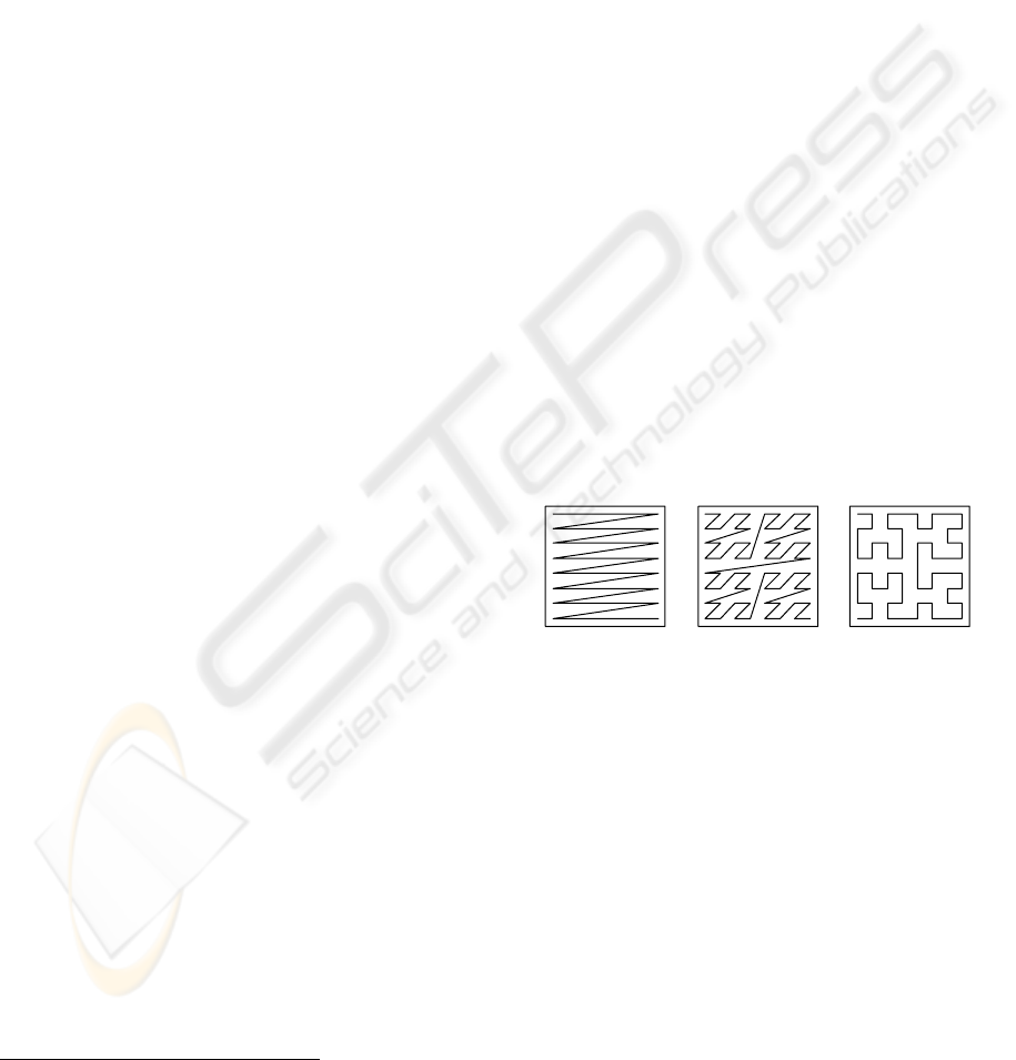
Examples for space filling curves include the
lexicographic-, Z- or Hilbert-order (cf. Figure 2),
with the Hilbert-order generating the least intervals
per object (Faloutsos C. et Al., 1989) (Jagadish H.
V., 1990) but being also the most complex linear
lexicographic order Hilbert-orderZ-order
Figure 2. Examples of space-filling curves in the
two-dimensional case.
O 2
IN
d
×∈
ρ:IN
d
IN→
Figure 2: Examples of space-filling curves in the two-
dimensional case
EFFICIENT JOIN PROCESSING FOR COMPLEX RASTERIZED OBJECTS
21
ordering. As a good trade-off between redundancy
and complexity, we use the Z-order throughout this
paper.
The resulting sequence of intervals, representing a
high resolution spatially extended object, often
consists of very short intervals connected by short
gaps. Experiments suggest that both gaps and
intervals obey an exponential distribution (Kriegel
H., 2003). In order to overcome this obstacle, it
seems promising to pass over some “small” gaps in
order to obtain much less intervals, which we call
gray intervals.
In the remainder of this section, we will introduce a
cost-based decompositioning algorithm which aims
at finding an optimal trade-off between replicating
and non-replicating approximations. In Section 2.1,
we first introduce our gray intervals formally, and
show how they can be integrated into an object
relational database system (ORDBMS). In Section
2.2, we discuss why it is beneficial to store the gray
intervals in a compressed way. In Section 2.3, we
introduce a cost-model for object decompositioning,
and introduce, in Section 2.4, the corresponding
cost-based decompositioning algorithm.
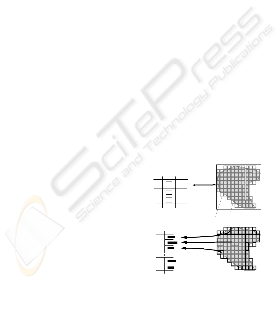
2.1 Gray intervals
Intuitively, a gray interval (cf. Figure 3) is a covering
of one or more ρ-order-values, i.e. integer values
resulting from the application of a space filling curve
ρ to a rasterized object (id, {v
1
, ..., v
n
}), where the
gray interval may contain integer values which are
not in the set {ρ(v
1
), ...,ρ(v
n
)}.
Definition 2 (gray interval, gray interval sequence)
Let (id, {v
1
, ..., v
n
}) be a rasterized object and
be a space filling curve. Furthermore, let W = {(l,
u), l ≤ u}⊆IN
2
be the domain of intervals and let b
1
=
(l
1
, u
1
), …, b
n
= (l
n
, u
n
)∈ W be a sequence of
intervals with u
i
+ 1 < l
i+1
, representing the set
{ρ(v
1
), ...,ρ(v
n
)}. Moreover, let m ≤ n and let i
0
, i
1
,
i
2
, …, i
m
∈ IN such that 0 = i
0
< i
1
< i
2
< …< i
m
= n
holds. Then, we call O
gray
= (id, <
, …, >) a gray interval sequence of
cardinality m. We call each
of the j = 1, …, m groups
of
O
gray
a gray interval I
gray
.
In Table 1, we introduce operators for a gray interval
I
gray
= <(l
r
,u
r
),…, (l
s
,u
s
)>. Figure 3 demonstrates the
values of some of these operators for a sample set of
gray intervals.
Storage of gray intervals. As indicated in Figure
1b, the approximations, i.e. the gray intervals, are
organized in auxiliary relations. We map the gray
intervals to the complex attribute data of the relation
GrayIntervals which is in Non-First-Normal-Form
(NF
2
) (cf. Figure 3). It consists of the hull H(I
gray
)
and a BLOB containing the byte sequence B(I
gray
)
representing the exact geometry. Important
advantages of this approach are as follows: First, the
hulls H(I
gray
) of the gray intervals can be used in a
fast filter step. Furthermore, we use the ability to
store the content of a BLOB outside of the table.
Therefore the column B(I
gray
) contains a BLOB
locator. This enables us to access the possibly huge
BLOB content only if it is required and not auto-
matically at the access time of H(I
gray
). In the next
section we discuss how the I/O cost of BLOBs can
be reduced by applying compression techniques.
2.2 Compression of gray intervals
In this section, we motivate the use of packers, by
showing that B(I
gray
) contains patterns. Therefore,
B(I
gray
) can efficiently be shrunken by using data
compressors. Furthermore, we discuss the properties
which a suitable compression algorithm should
fulfill. In the following, we give a brief presentation
of a new effective packer which is promising for our
approach. It exploits gaps and patterns included in
the byte sequence B(I
gray
) of our gray interval I
gray
.
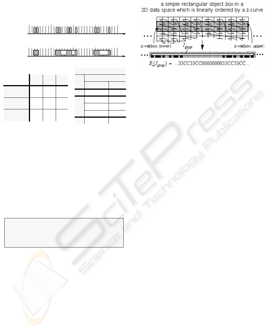
Patterns. To describe a rectangle in a 2D vector
space, we only need 4 numerical values, e.g. we need
two 2-dimensional points. In contrast to the vector
representation, an enormous redundancy might be
contained in the corresponding voxel sequence of an
object, an example is shown in Figure 4. As space
filling curves, in particular the Z-order, enumerate
the data space in a structured way, we can find such
“structures” in the resulting voxel sequence
representing simply shaped objects. We can pinpoint
the same phenomenon not only for simply shaped
parts but also for more complex real-world spatial
parts. Assuming we cover the whole voxel sequence
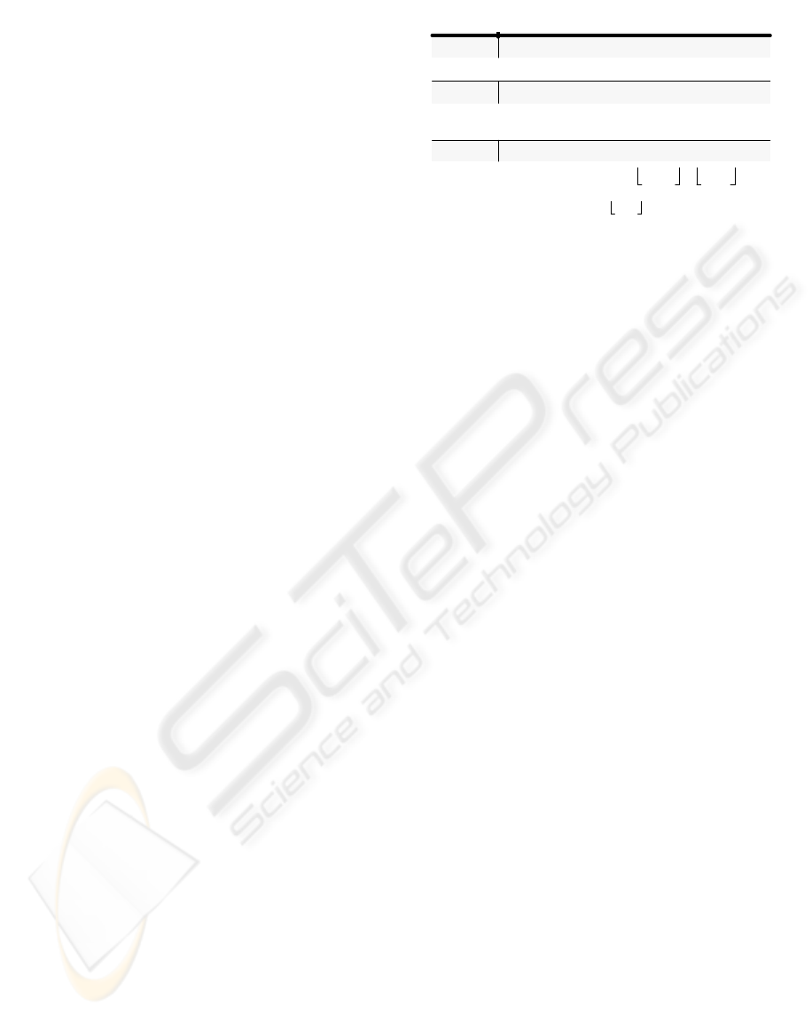
Operator Description and Definition
H
(I
gray
)
hull
(l
r
,u
s
)
G
(I
gray
)
maximum gap
{
B (I
gray
)
byte sequence
<s
0
, .., s
n
> where 0 ≤ s
j
< 2
8
,
Table 1. Operators on gray intervals.
0
r
s
=
max l
i
u
i 1–
–1– ir1 … s,,+=,{}else
n
u
s
8
⁄
l
r
8
⁄
–
=
s
i
2
7 k–
0
k 0=
7
∑
if l
t
,u
t
()∃ :l
t
l
r
8⁄ 8⋅ 8iku
t
rts≤≤,≤++≤
otherwise
=
ρ:IN
d
IN→
b
i
0
1+
,...,b
i
1
〈〉
b
i
m 1–
1+
,...,b
i
m
〈〉
b
i
j 1–
1+
,...,b
i
j
〈〉
Table 1: Operators on gray intervals
ICEIS 2005 - HUMAN-COMPUTER INTERACTION
22
of an object id by one interval, i.e. O
gray
= (id,
_I
gray
_), and survey its byte representation B(I
gray
) in
a hex-editor, we can notice that some byte sequences
occur repeatedly. For more details about the
existence of patterns in B(I
gray
) we refer the reader to
(Kunath P., 2002).
We will now discuss how these patterns can be used
for the efficient storage of gray intervals.
Compression rules. A voxel set belonging to a gray
interval I
gray
can be materialized and stored in a
BLOB in many different ways. A good
materialization should consider two “compression
rules”:
A good join response behavior is based on the fulfill-
ment of both aspects. The first rule guarantees that
the I/O cost are relatively small whereas
the second rule is responsible for low CPU cost
. . The overall cost
for the evaluation of a BLOB is composed of both
parts. A good behavior related to an efficient
retrieval and evaluation of B(I
gray
) depends on the
fulfillment of both rules.
As we will show in our experiments, it is very
important for a good retrieval- and evaluation-
behavior to find a well-balanced way between these
two compression rules.
Spatial compression techniques. In this section, we
look at a new specific compression technique, which
is designed for storing the voxel set of a gray interval
in a BLOB. According to our experiments, the new
data compressor outperforms popular standard data
compressors such as BZIP2 (Burrow M. et Al.,
1994).
Quick Spatial Data Compressor (QSDC). The
QSDC algorithm is especially designed for high
resolution spatial data and includes specific features
for the efficient handling of patterns and gaps. It is
optimized for speed and does not perform time
intensive computations as for instance Huffman
compression. QSDC is a derivation of the LZ77
technique (Lempel A. et Al., 1977).
QSDC operates on two main memory buffers. The
compressor scans an input buffer for patterns and
gaps. QSDC replaces the patterns with a two- or
three-byte compression code and the gaps with a
one- or two-byte compression code. Then it writes
the code to an output buffer. QSDC packs an entire
BLOB in one piece, the input is not split into smaller
chunks. At the beginning of each compression cycle
QSDC checks if the end of the input data has been
reached. If so, the compression stops. Otherwise
another compression cycle is executed. Each pass
through the cycle adds one item to the output buffer,
either a compression code or a non-compressed
character. Unlike other data compressors, no
checksum calculations are performed to detect data
corruption because the underlying ORDBMS ensures
data integrity.
The decompressor reads compressed data from an
input buffer, expands the codes to the original data,
and writes the expanded data to the output buffer.
For more details we refer the reader to (Kunath P.,
2002), where it was shown that QSDC is more
suitable for spatial query processing than zlib
(Lempel A. et Al., 1977) due to the higher (un)pack
speed and an almost as high compression ratio.
Rule 1: As little as possible secondary storage
should be occupied.
Rule 2: As little as possible time should be needed
for the (de)compression of the BLOB.
cost
BLOB
cost
BLOB
I/O
cost
BLOB
CPU
+=
Figure 3. Gray interval sequence.
gray intervals
gray interval
operators
I
1
I
2
I
3
hull:
H( I
x
)
[578,
579]
[586,
593]
[600,
605]
maximum gap:
G( I
x
)
0 2 3
byte sequence:
B( I
x
)
’30’ ’33 40’ ’C4’
GrayIntervals
id
data
H(I
x
) B(I
x
)
... ... ...
E
[578, 579] ’30’
[586, 593] ’3340’
[600, 605] ’C4’
... ... ...
I
1
I
2
I
3
576 584
592
600
608
(obtained by splitting at selected gaps)
576
584 592
600 608
set of
object voxels
cost
BLOB
I/O
cost
BLOB
I/O
Figure 4: Pattern derivation by linearizing a rasterized
object using a space-filling curve (Z-order).
Figure 3: Gray interval sequence
EFFICIENT JOIN PROCESSING FOR COMPLEX RASTERIZED OBJECTS
23
2.3 Cost model
For our decompositioning algorithm we take the esti-
mated join cost between a gray interval I
gray
and a
join-partner relation T into account. Let us note that
T can be either of the tables R or S (cf. Figure 1a), or
any temporary table containing derived information
from the original tables R and S (cf. Figure 1b). The
overall join cost cost
join
for a gray interval I
gray
and a
join-partner relation T are composed of two parts,
the filter cost cost
filter
and the refinement cost
cost
refine
:
cost
join
(I
gray
,T) = cost
filter
(I
gray
,T) + cost
refine
(I
gray
,T).
The question at issue is, which decompositioning is
most suitable for an efficient join processing. A good
decompositioning should take the following
“decompositioning rules” into consideration:
The first rule guarantees that cost
filter
is small, as
each gray interval I
gray,T
of the join-partner relation T
has to be loaded from disk (BLOB content excluded)
and has to be evaluated for intersection with respect
to its hull.
In contrast, the second rule guarantees that many
unnecessary candidate tests of the refinement step
can be omitted, as the number and size of gaps
included in the gray intervals, i.e. the approximation
error, is small. Finally, the third rule guarantees that
a candidate test can be carried out efficiently. Thus,
Rule 2 and Rule 3 are responsible for low cost
refine
. A
good join response behavior results from an
optimum trade-off between these decompositioning
rules.
Filter cost. The cost
filter
(I
gray
,T) can be computed by
the expected number of gray intervals I
gray,T
of the
join partner relation T. We penalize each intersection
test by a constant c
f
which reflects the cost related to
the access of one gray interval I
gray,T
and the
evaluation of the join predicate for the pair
(H(I
gray
),H(I
gray,T
)):
cost
filter
(I
gray
,T) = N
gray
(T) . c
f
,
where N
voxel
(T) (number of voxels) ≥ N
gray
(T)
(number of gray intervals) ≥ N
object
(T) (number of
objects) holds for the join-partner relation. The value
of the parameter c
f
depends on the used system.
Refinement cost. The cost of the refinement step
cost
refine
is determined by the selectivity of the filter
step. For each candidate pair resulting from the filter
step, we have to retrieve the exact geometry B(I
gray
)
in order to verify the intersection predicate.
Consequently, our cost-based decompositoning
algorithm is based on the following two parameters:
• Selectivity σ
filter
of the filter step.
• Evaluation cost cost
eval
of the exact geometries.
The refinement cost of a join related to a gray
interval I
gray
can be computed as follows:
cost
refine
(I
gray
, T) = N
gray
(T) · σ
filter
(I
gray
,T) · cost
eval
(I
gray
).
In the following paragraphs, we show how we can
estimate the selectivity of the filter step σ
filter
and the
evaluation cost cost
eval
.
Selectivity estimation. We use simple statistics of
the join-partner relation T to estimate the selectivity
σ
filter
(I
gray
,T). In order to cope with arbitrary interval
distributions, histograms can be employed to capture
the data characteristics at any desired resolution. We
start by giving the definition of an interval
histogram:
Definition 3 (interval histogram).
Let D= [0,2
h
–1] be a domain of interval bounds,
h≥1. Let the natural number ν∈IN denote the
resolution, and β
ν
= (2
h
–1)/ν be the corresponding
bucket size. Let b
i,ν
= [1+(i–1)·β
ν
,1+i·β
ν
) denote the
span of bucket i, i∈{1, …, ν}. Let further T= {(l,u),
l
≤
u} ⊆ D
2
be a database of intervals. Then, IH(T,ν)
= (n
1
,…, n
ν
)∈IN
ν
is called the interval histogram on
T with resolution ν, iff for all i∈{1,.., ν}:
n
i
= |{ψ ∈ T | ψ intersects b
i,ν
}|
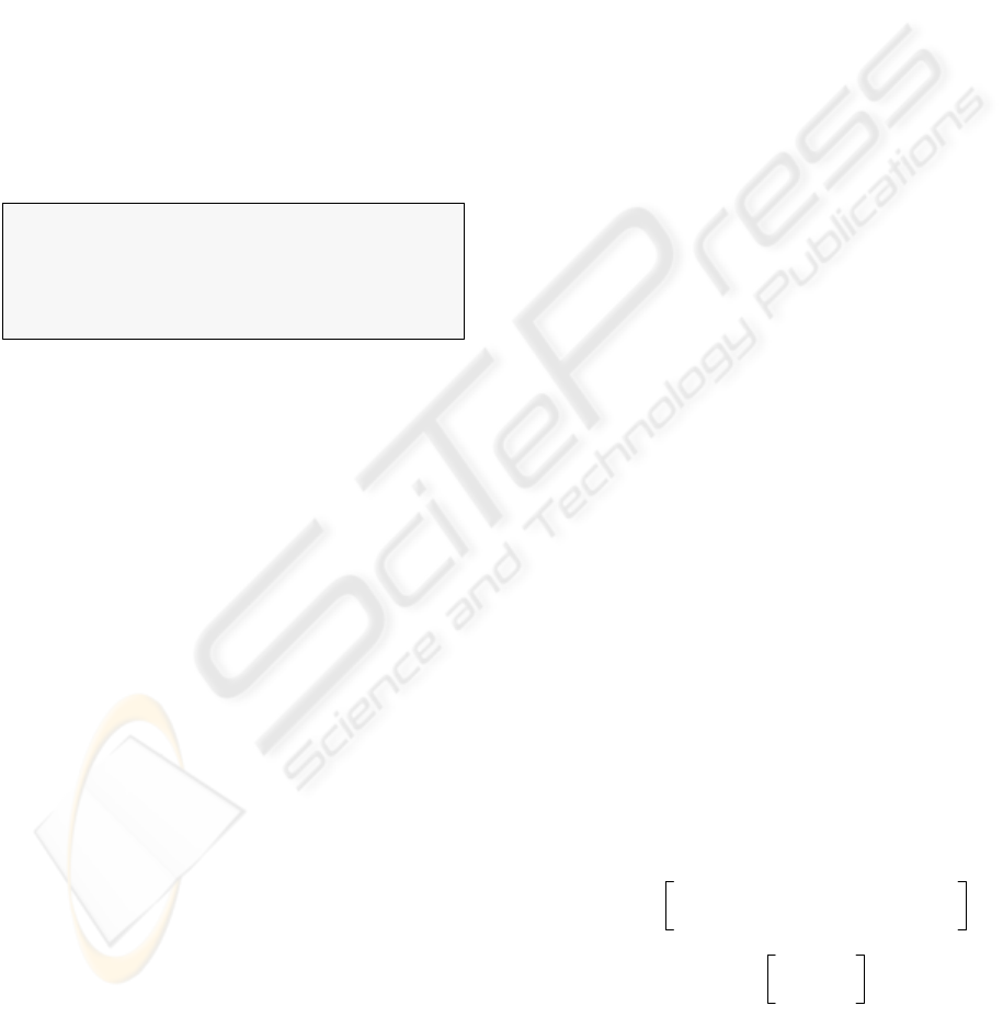
The selectivity σ
filter
(I
gray
,T) related to a gray interval
I
gray
can be determined by using an appropriate
interval histogram IH(T,ν) of the join partner
relation T. Based on IH(T, ν), we compute a
selectivity estimate by evaluating the intersection of
I
gray
with each bucket span b
i,ν
(cf. Figure 5).
Definition 4 (histogram-based selectivity estimate).
Given an interval histogram IH(T,ν)=(n
1,
...,n
ν
) with
bucket size β, we define the histogram-based
selectivity estimate σ
filter
(I
gray
,T), 0≤σ
filter
(I
gray
,T) ≤1
by the following formula:
σ
filter
(I
gray
,T)=
where overlap returns the intersection length of two
intersecting intervals, and 0, if the intervals are
disjoint.
Rule 1: The number of gray intervals should be small.
Rule 2: The approximation error of all
gray
intervals
should be small.
Rule 3: The
gray intervals
should allow an efficient
evaluation of the contained voxels.
overlap H I
gray
()b
i ν,
,()
β
---------------------------------------------------------
n
i
⋅
i 1=
ν
∑
n
i
i 1=
ν
∑
---------------------------------------------------------------------
ICEIS 2005 - HUMAN-COMPUTER INTERACTION
24
Note that long intervals may span multiple histogram
buckets. Thus, in the above computation, we
normalize the expected output to the sum of the
number n
i
of intervals intersecting each bucket i
rather than to the original cardinality n of the
database.
BLOB-Evaluation cost. The evaluation of the
BLOB content requires to load the BLOB from disk
and decompress the data. Consequently, the
evaluation cost depends on both the size L(I
gray
) of
the uncompressed BLOB and the size L
comp
(I
gray
) <<
L(I
gray
) of the compressed data. Additional, the
evaluation cost cost
eval
depend on a constant
c
I/O
loadrelated to the retrieval of the BLOB from
secondary storage, a constant c
cpu
decomprelated to
the decompression of the BLOB, and a constant
c
cpu
testrelated to the intersection test. The cost
c
cpu
decompand c
I/O
load heavily depend on how we
organize B(I
gray
) within our BLOB, i.e. on the used
compression algorithm. A highly effective but not
very time efficient packer, e.g. BZIP2, would cause
low loading cost but high decompression cost. In
contrast, using no compression technique, leads to
very high loading cost but no decompression cost.
Our QSDC (cf. Section 2.2) is an effective and very
efficient compression algorithm which yields a good
trade-off between the loading and decompression
cost. Finally, c
cpu
test solely depend on the used
system. The overall evaluation cost are defined by
the following formula:
Join cost. To sum up the join cost cost
join
(I
gray
)
related to a gray interval I
gray
and a join-partner
relation T can be expressed as follows:
cost
join
(I
gray
,T) =
N
gray
(T)·(c
f
+ σ
filter
(I
gray
,T) ·cost
eval
(I
gray
)),
where the filter selectivity and BLOB-evaluation cost
are computed as described in Section 2.3.
2.4 Decompositioning algorithm
For each rasterized object, there exist many different
possibilities to decompose it into a gray interval
sequence.
Based on the formulas for join cost related to a gray
interval I
gray
and a join-partner relation T, we can
find a cost optimum decompositioning algorithm. In
this section, we present a greedy algorithm with a
guaranteed worst-case runtime complexity of O(n)
which produces decompositions helping to
accelerate the query process considerably.
For fulfilling the decompositioning rules presented
in Section 2.3, we introduce the following cost-based
decompositioning algorithm for gray intervals, called
CoDec (cf. Figure 6). CoDec is a recursive top-down
algorithm which starts with a gray interval I
gray
initially covering the complete object. In each step of
our algorithm, we look for the longest remaining
gap. We carry out the split at this gap, if the
estimated join cost caused by the decomposed
intervals is smaller than the estimated cost caused by
our input interval I
gray
. The expected join cost
cost
join
(I
gray
,T) can be computed as described above.
Data compressors which have a high compression
rate and a fast decompression method, result in an
early stop of the CoDec algorithm generating a small
number of gray intervals. Let us note that the
inequality “cost
gray
>cost
dec
” in Figure 6 is
independent of N
gray
(T), and thus N
gray
(T) is not
required during the decompositioning algorithm.
3 JOIN ALGORITHM
In contrast to the last section, where we focused on
building the object approximations and organizing
them within the database, we introduce a concrete
Figure 6. Decompositioning algorithm CoDec.
CoDec (I
gray
, IH(T,v), T) {
interval_pair := split_at_maximum_gap(I
gray
);
I
left
:= interval_pair.left;
I
right
:= interval_pair.right;
cost
gray
:= cost
join
(I
gray
,T);
cost
dec
:= cost
join
(I
left
,T) + cost
join
(I
right
,T);
if cost
gray
> cost
dec
then
return CoDec (I
left
,IH(T,v),T) ∪ CoDec (I
right
,IH(T,v),T);
else
return I
gray
; }
t
eval
I
gray
() =cos
L
comp
I
gray
()c
load
I/O
⋅ LI
gray
()c
decomp
cpu
c
test
cpu
+()⋅+
Figure 7: Selectivity estimation on an interval
histogram
Figure 6: Decompositioning algorithm CoDec.
EFFICIENT JOIN PROCESSING FOR COMPLEX RASTERIZED OBJECTS
25
join algorithm based on CoDec in this section. Our
join algorithm is based on the worst-case optimal
interval join algorithm described in (Arge L. et Al.,
1998) and on the cost-based decompositioning
approach described in the last section. In the
following, we consider R and S as input relations (cf.
Figure 1a). The join algorithm is performed in plane-
sweep fashion where we approximate each object o
by the z-values of its mbr, i.e. an object is
approximated by one gray interval [z-
val(mbr.lower), z-val(mbr.upper)] (cf. Figure 4). We
process these gray intervals according to their
starting points. Note that we assume that we have
access to the mbrs, without accessing the detailed
object description stored in a file (cf. Figure 1a).
As we cannot assume that the sweep-line status com-
pletely fits in memory, we additionally use two auxil-
iary relations R’ and S’ (cf. Figure 1b) to hold the
actual sweep-line status on disk. Both relations R’
and S’ follow the NF
2
of the relation GrayIntervals
(cf. Figure 3).
In order to adjust the object approximations to the
data distribution of the respective join-partner
relation, we apply our decomposition algorithm (cf.
Section 2.4). For the computation of the data
distribution we use interval histograms where we
perform the decomposition in two steps employing
two different interval histograms for each data set.
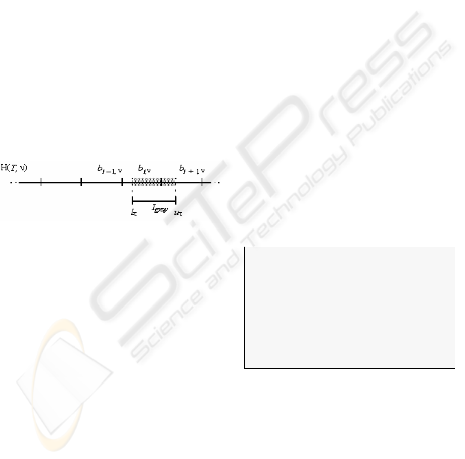
The interval histograms IH
Sweep,R’
and IH
Sweep,S’
represent the data distribution within the actual
sweep-line status and are dynamically updated. The
other interval histograms IH
All,R
and IH
All,S
represent
the overall data distribution, derived from R and S
and are static. In the following, we assume that all
interval histograms have the same resolution v, so
that their bucket borders are congruent. An example
is shown in Figure 7. The figure shows for relation R
that only the decomposed gray intervals left from the
actual sweep-line status contribute to the histogram
IH
Sweep,R’
whereas IH
All,R
takes all one value gray
intervals into consideration.
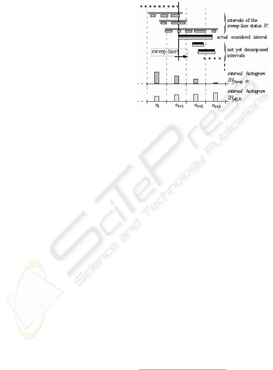
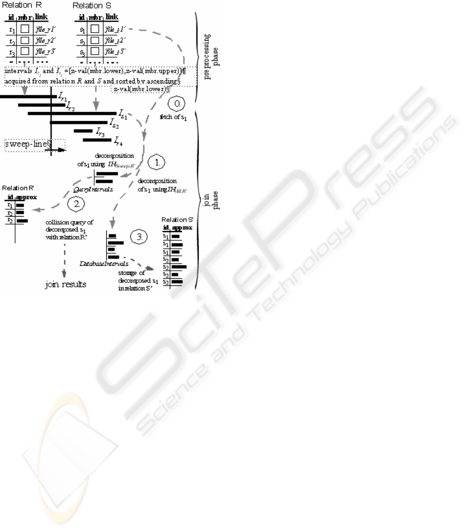
Our sort-merge join algorithm consists of two phases
where the second phase in turn consists of three steps
which are performed for each object. The complete
join algorithm described in the following is depicted
in Figure 8:
Preprocessing phase. Initially, we gather the
statistics about the data distribution of R and S where
each object o is approximated by the z-values of its
mbr, i.e. o is approximated by one gray interval [z-
val(mbr.lower), z-val(mbr.upper)]. Note that this
preprocessing step can be carried out efficiently, as
we do not have to access the complex object
representations. The statistical data distribution of
the gray intervals is stored in two interval histograms
IH
All,R
and IH
All,S
. Next, we order the union of both
relations R and S according to the value z-
val(mbr.lower) of their objects.
Join phase. We apply a plane sweep algorithm to
walk through this sorted list containing gray intervals
of both relations R and S. The event points of this
algorithm are the starting points of the gray intervals.
Each encountered interval I
gray
= (l, u) from relation
S is now processed according to the following four
steps
2
:
Step 0: First, we carry out a coarse filter step. We
test whether I
gray
can possibly intersect a gray
interval of relation R by exploiting the statistical
information stored in IH
All,R
. If there cannot be any
intersection as I
gray
spans only empty buckets of
IH
All,R
, we are finished for this object. Otherwise, the
exact object description, i.e. the content of the file, is
loaded for I
gray
and we continue with the Step 1.
Step 1: I
gray
is decomposed based on the data
distribution of the actual sweep-line status of the
relation R’, i.e. by applying IH
Sweep,R’
, and stored in a
temporary list QueryIntervals. This first
2 The intervals for R are treated similarly.
Figure 7: Intervals stemming from R and the
corresponding histograms
IH
Sweep,R’
and IH
All,R
.
ICEIS 2005 - HUMAN-COMPUTER INTERACTION
26
decompositioning aims at finding an optimum
decompositioning for querying the already
decomposed intervals of relation R stored in R’.
In the same step we also decompose I
gray
applying
the statistics IH
All,R
and buffer the result in another
temporary list, called DatabaseIntervals. This
decompositioning anticipates an optimum
approximation for assumed gray query intervals of
relation R, which have not yet been processed.
Step 2: The temporary list QueryIntervals is used as
query object for the relation R’. We report all objects
having a gray interval I’
gray
stored in R’ which
intersects at least one of the decompositions of I
gray
.
These intersection queries can efficiently be carried
out by following the approach presented in (Kriegel
H., 2003).
Step 3: The decomposed intervals of the temporary
list DatabaseIntervals are stored in a compressed
way in the temporary relation S’. Finally, we have to
update the interval histogram IH
Sweep,S’
.
Note that this sort-merge join variant does not
require any duplicate elimination. Furthermore, the
main memory footprint of the presented join
algorithm is negligible because we do not keep the
sweep-line status in main-memory. Even if we kept it
in main memory, the use of suitable data
compressors would reduce the BLOB sizes of the
tables R’ and S’ considerably leading to a rather
small main memory-footprint (cf.
Section 4).
4 EXPERIMENTAL EVALUATION
In this section, we evaluate the performance of our
approach with a special emphasis on different
decompositioning algorithms in combination with
various data compression techniques DC. We used
the following data compressors: no compression
(NOOPT), the BZIP2 approach (Seward J.) and the
QSDC approach. Furthermore, we decomposed
object voxels into gray intervals following two
decompositioning algorithms, called MaxGap and
CoDec.
MaxGap. This decompositioning algorithm tries to
minimize the number of gray intervals while not
allowing that a maximum gap G(I
gray
) of any gray
interval I
gray
exceeds a given MAXGAP parameter.
By varying this MAXGAP parameter, we can find the
optimum trade-off between the first two opposing
decompositioning rules of Section , namely a small
number of gray intervals and a small approximation
error of each of these intervals. A one-value interval
approximation is achieved by setting the MAXGAP
parameter to infinite.
CoDec. We decomposed the voxel sets according to
our cost- based decompositioning algorithm CoDec
(cf. Section 2.4), where we set the resolution of the
used histograms to 100 buckets.
Let us note, that the decompositioning based on
MaxGap(DC) does not depend on DC or any
statistical information about the data distribution,
whereas CoDec(DC) takes the actual data
compressor DC and the actual data distribution into
account for performing the decompositioning.
The refinement-step evaluation of the intersect()
routine was delegated to a DLL written in C. All
experiments were performed on a Pentium 4/2600
machine with IDE hard drives. The database block
cache was set to 500 disk blocks with a block size of
8 KB and was used exclusively by one active
session.
Test data sets. The tests are based on two test data
sets CAR (3D CAD data) and SEQUOIA (subset of
2D GIS data representing woodlands derived from
Figure 8: Two-phase sort-merge join
EFFICIENT JOIN PROCESSING FOR COMPLEX RASTERIZED OBJECTS
27
the SEQUOIA 2000 benchmark (Stonebraker M.,
1993)). The first test data set was provided by our
industrial partner, a German car manufacturer, in
form of high resolution rasterized three-dimensional
CAD parts.
data set # voxels # objects size of data space
CAR 14x106 200 233 cells
SEQUOIA 32x106 1100 234 cells
In both cases, the Z-order was used as a space filling
curve to enumerate the voxels. Both test data sets
consist of many short black intervals and short gaps
and only a few longer ones.
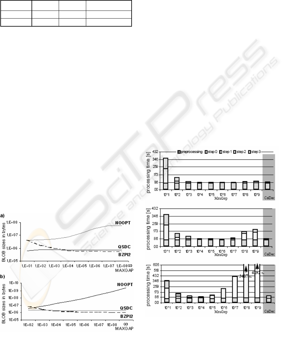
Compression Techniques. Figure 9 shows the
different storage requirements of the BLOBs with
respect to the different data compression techniques
for the materialized gray intervals. For high
MAXGAP values, the BZIP2 approach yields very
high compression rates, i.e. compression rates up to
1:100 for the SEQUOIA dataset and 1:500 for the
CAR dataset. Note that the higher compression rates
for the CAR dataset are due to fact that it is a 3D
dataset, whereas the SEQUOIA dataset is a 2D
dataset. This additional dimension leads to an
enormous increase of the BLOB sizes making
suitable compression techniques indispensable. On
the other hand, due to a noticeable overhead, the
BZIP2 approach occupies even more secondary
storage space than NOOPT for small MAXGAP
values. Contrary, the QSDC approach yields good
results over the full range of the MAXGAP
parameter. Using the QSDC compression technique,
we achieve low I/O cost for storing (Step3) and
fetching (Step2) the BLOBs which drastically
enhances the efficiency of the join process.
Decomposition-Based Join Algorithm. In this para-
graph, we want to investigate the runtime behavior of
our decomposition- based join algorithm presented
in Section . We performed the intersection join over
two relations, each containing approximately a half
of the parts from the CAR dataset. We took care that
the data of both relations have similar
characterizations with respect to the object size and
distribution. Similarly, the intersection join is
performed on parts of the SEQUOIA data set which
is divided into two relations, consisting of
deciduous-forest and mixed-forest areas.
Dependency on the MAXGAP parameter. In Figure
10 and Figure 11 it is shown how the response time
for the intersection join, including the preprocessing
step, depends on the MAXGAP parameter, if we use
no cache, i.e. the temporary relations R’ and S’ are
not kept in main memory. The preprocessing time,
i.e. the time for the creation of the statistics, is
negligible. Step 0 of the join phase, i.e. the loading
of the exact object descriptions, is rather high and
Figure 9: Storage requirements for the BLOB:
a) SEQUOIA, b) CAR
Figure 10: Comparison between MaxGap and CoDec
grouping based on different compression algorithms
(main memory cache disabled) (SEQUOIA):
ICEIS 2005 - HUMAN-COMPUTER INTERACTION
28
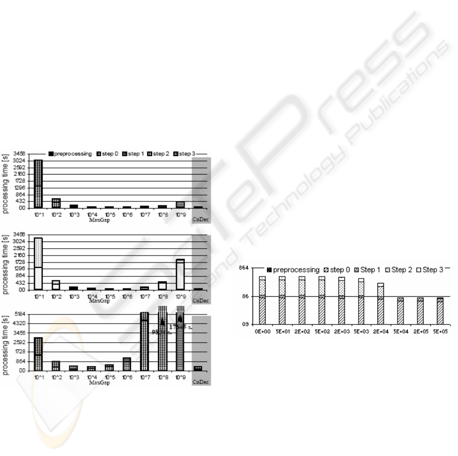
almost constant w.r.t. a varying MAXGAP parameter.
On the other hand, Step 1, the statistic-based
decompositioning of our gray intervals is very cheap
for our CoDec algorithm, and for the Maxgap-
approach it is not needed. Step 2, i.e. the actual
intersection query, heavily depends on the used
MAXGAP-value and the applied compression algo-
rithm.
For small MAXGAP-values we have rather high cost
for all compression techniques as the number of used
gray query intervals is very high. For high MAXGAP
values we only have high cost, if we use the NOOPT
compression approach. On the other hand, if we use
our QSDC-approach the actual cost for the
intersection queries stay low, as we have rather low
I/O cost and are able to efficiently decompress the
gray intervals. If we use the BZIP2-approach for
high MAXGAP-values, we also have low I/O cost but
higher CPU cost than for the QSDC-approach. Due
to these rather high CPU cost, the BZIP2 approach
performs worse than the QSDC-approach. The
incidental cost for Step 3, i.e. the storing of the
decomposed gray intervals in temporary relations,
can be explained similar to the cost for Step 2. Note
that the cost for Step 2 and Step 3 are smaller if we
allow a higher main memory footprint.
For MAXGAP-values around 10
6
our join algorithm
works most efficiently for the QSDC and BZIP2
compression approaches. Note that our CoDec-based
decompositioning yields results quite close to these
optimum ones. For the NOOPT-approach the best
possible runtime can be achieved for MAXGAP-
values around 10
4
. Again, the runtime of our join
based on the CoDec-algorithm is close to this
optimum one, justifying the suitability of our
grouping algorithm.
Dependency on the available main memory. Figure
12 shows for the CAR dataset how the runtime of the
complete join algorithm depends on the available
main-memory. We keep as much as possible of the
sweep-line status in main memory instead of
immediately externalizing it. The figure shows that
for uncompressed data Step 2 and Step 3 (cf. Figure
8) are very expensive if the available main memory
is limited. If we use our CoDec algorithm without
any compression, we need 50 MB or more to get the
best possible runtime. If we use CoDec in
combination with the QSDC approach, we only need
about 2 MB to get the best runtime. The two
optimum runtimes are almost identical because one
of the main design goals of the QSDC was high
unpack speed. Note that already by a main memory
footprint of 0 KB, i.e. the sweep-line status cache is
disabled, the QSDC approach achieves runtimes
close to the optimum ones demonstrating a high
compression ratio of the QSDC.
Figure 13 for the CAR dataset and Figure 14 for the
SEQUOIA dataset show the influence of the
available main memory for one-value interval
approximations, i.e. O
gray
= (id, I
gray
), and gray
approximations formed by our CoDec algorithm.
The one-value interval approximations produce more
false hits resulting in higher refinement cost. Note,
that one-value interval approximations of
uncompressed data cannot be kept in main memory
even if allowing a main memory footprint of up to
1.5 GB. Furthermore the figures demonstrate the
superiority of the QSDC approach compared to the
Figure 11: Comparison between MaxGap and CoDec
grouping based on different compression algorithms
(main memory cache disabled)(CAR).
Figure 12: Sort-merge join performance for different
cache sizes of the sweep-line status (
CAR dataset).
left column:
CoDec(NOOPT),
right column:
CoDec(QSDC)
EFFICIENT JOIN PROCESSING FOR COMPLEX RASTERIZED OBJECTS
29
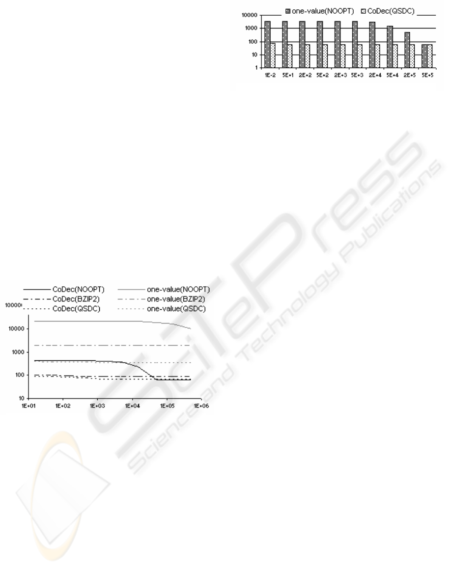
BZIP2 approach independent of the available main
memory. This superiority is due to the high (un)pack
speed of the QSDC and a comparable compression
ratio.
To sum up, our cost-based decompositioning
algorithm CoDec together with our QSDC approach
leads to a very efficient sort-merge join while
keeping the required main memory small. For
reasonable main memory sizes we achieve an
acceleration by more than one order of magnitude
for the SEQUOIA dataset and by more than two
orders of magnitude for the CAR dataset compared
to the traditionally used non-compressed one-value
approximations.
5 CONCLUSIONS
Complex rasterized objects are indispensable for
many modern application areas such as geographical
information systems, digital-mock-up, computer-
aided design, medical imaging, molecular biology, or
real-time virtual reality applications as for instance
haptic rendering. In this paper, we introduced an
efficient intersection join for complex rasterized
objects which uses a cost-based decompositioning
algorithm generating replicating compressed object
approximations. The cost model takes the actual data
distribution reflected by statistical information and
the used packer characteristics into account. In order
to generate suitable compressed approximations, we
introduced a new spatial data compressor QSDC
which achieves good compression ratios and high
unpack speeds. In a broad experimental evaluation
on real-world geographical and 3D CAD datasets,
we demonstrated the efficiency of our new spatial
join algorithm for complex rasterized objects.
In our future work, we want to apply our new join-
method to virtual reality applications, where the
efficient management of complex rasterized objects
is also decisive.
REFERENCES
Arge L., Procopiuc O., Ramaswamy S., Suel T., Vitter
J.S.: Scalable Sweeping-Based Spatial Join, In Proc.
of the VLDB Conference, 1998, 570-581.
Burrows M., Wheeler D. J.: A Block-sorting Lossless Data
Compression Algorithm, Digital Systems Research
Center Research Report 124, 1994.
Faloutsos C., Roseman S.: Fractals for Secondary Key
Retrieval. In Proc. ACM PODS, 1989, 247-252.
Gaede V.: Optimal Redundancy in Spatial Database
Systems, In Proc. 4th Int. Symp. on Large Spatial
Databases, 1995, 96-116.
Jagadish H. V.: Linear Clustering of Objects with Multiple
Attributes. In Proc. ACM SIGMOD, 1990, 332-342.
Kriegel H.-P., Pfeifle M., Pötke M., Seidl T.: Spatial
Query Processing for High Resolutions. Database
Systems for Advanced Applications (DASFAA), 2003.
Kunath P.: Compression of CAD-data, Diploma thesis,
University of Munich, 2002.
Lempel A., Ziv J.: A Universal Algorithm for Sequential
Data Compression. IEEE Transactions on Information
Theory, Vol. IT-23, No. 3, 1977, 337-343.
Orenstein J. A.: Spatial Query Processing in an Object-
Oriented Database System, In Proc. of the ACM
SIGMOD Conference, 1986, 326-336.
Seward J.: The bzip2 and libbzip2 official home page.
http://sources.redhat.com/bzip2.
Stonebraker M., Frew J., Gardels K., Meredith J.: The
SEQUOIA 2000 Sorage Benchmark. In Proc. ACM
SIGMOD Int. Conf. on Management of Data: 1993
Figure 13: Overall sort-merge join performance for
different cache sizes of the sweep-line status (
CAR
dataset).
Figure 14: Sort-merge join performance for
different cache sizes of the sweep-line status
(
SEQUOIA dataset)
ICEIS 2005 - HUMAN-COMPUTER INTERACTION
30
