
CONSTRUCTION OF DECISION TREES USING DATA CUBE
Lixin Fu
383 Bryan Bldg., University of North Carolina at Greensboro, Greensboro, NC 27402-6170, USA
Keywords: Classification, Decision Trees, Data Cube
Abstract: Data classification is an important problem in data m
ining. The traditional classification algorithms based
on decision trees have been widely used due to their fast model construction and good model
understandability. However, the existing decision tree algorithms need to recursively partition dataset into
subsets according to some splitting criteria i.e. they still have to repeatedly compute the records belonging
to a node (called F-sets) and then compute the splits for the node. For large data sets, this requires multiple
passes of original dataset and therefore is often infeasible in many applications. In this paper we present a
new approach to constructing decision trees using pre-computed data cube. We use statistics trees to
compute the data cube and then build a decision tree on top of it. Mining on aggregated data stored in data
cube will be much more efficient than directly mining on flat data files or relational databases. Since data
cube server is usually a required component in an analytical system for answering OLAP queries, we
essentially provide “free” classification by eliminating the dominant I/O overhead of scanning the massive
original data set. Our new algorithm generates trees of the same prediction accuracy as existing decision tree
algorithms such as SPRINT and RainForest but improves performance significantly. In this paper we also
give a system architecture that integrates DBMS, OLAP, and data mining seamlessly.
1 INTRODUCTION
Data classification is a process of building a model
from available data called training data set and
classifying the objects according to their attributes.
It is a well-studied important problem (Han and
Kamber 2001), and has many applications in
insurance industry, tax and credit card fraud
detection, medical diagnosis, etc.
The existing decision tree algorithm
s need to
recursively partition dataset into subsets physically
according to some splitting criteria. For large data
sets, building a decision tree this way requires
multiple passes of the original dataset, therefore, is
often infeasible in many applications. In this paper
we present a new approach of constructing decision
trees using pre-computed data cube.
Our main contributions in this paper include:
• designing a new decision tree classifier
b
uilt on data cube, and
• proposi
ng an architecture that takes the
advantages of above new algorithm and
integrates DBMS, OLAP systems, and data
mining systems seamlessly.
The remaining of the paper is organized as
fol
lows. The next section gives a brief summary of
the related work. In Sec. 3, statistics tree structures
and related data cube computation algorithms are
described as the foundation of later sections. An
architecture that integrates DBMS, OLAP, and data
mining functions is proposed in Sec. 4. Sec. 5
describes our new cube-based decision tree
classification algorithm called cubeDT. Evaluation
of cubeDT is given in Sec. 6. Lastly, we summarize
the paper, and discuss the directions of our related
future work.
2 BACKGROUND
Decision trees have been widely used in data
classification. As its precursor algorithm ID-3
(Quilan 1986), algorithm C4.5 (Quilan 1993)
generates a simple tree in a top-down fashion. Data
are partitioned into subsets recursively according to
best splitting criteria determined by highest
information gain until the partitions contain samples
of the same classes. For continuous attribute A, the
values are sorted and the midpoint v between two
values is considered as a possible split. The split
119
Fu L. (2005).
CONSTRUCTION OF DECISION TREES USING DATA CUBE.
In Proceedings of the Seventh International Conference on Enterprise Information Systems, pages 119-126
DOI: 10.5220/0002509801190126
Copyright
c
SciTePress

form is A ≤ v. For a categorical attribute, if its
cardinality is small, all subsets of its domain can be
candidate splits; otherwise, we can use a greedy
strategy to create candidate splits.
SLIQ (Mehta, Agrawal et al. 1996) and
SPRINT (Shafer, Agrawal et al. 1996) are more
recent decision-tree classifiers that address the
scalability issues for large data sets. Both use Gini
index as impurity function, presorting (for numerical
attributes), and breadth-first-search to avoid
resorting at each node. Both SLIQ and SPRINT are
still multi-pass algorithms for large data sets due to
the necessity of external sorting and out-of-memory
structures such as attribute lists.
Surajit et al. (Chaudhuri, Fayyad et al. 1999)
give a scalable classifier over a SQL database
backend. They develop a middleware that batches
query executions and stages data into its memory or
local files to improve performance. At its core is a
data structure called count table or CC table, a four-
column table (attribute-name, attribute-value, class-
value, count). Gehrke et al. give a uniform
framework algorithm RainForest based on AVC-
group (a data structure similar to CC tables but as
independent work) for providing scalable versions of
most decision tree classifiers without changing the
quality of trees (Gehrke, Ramakrishnan et al. 1998).
With usually much smaller sizes of CC tables or
AVC-group than the original data or attribute lists in
SPRINT, these two algorithms generally improve
the mining performance. However, they together
with all other classification algorithms (as far as we
know) including SLIQ and SPRINT still need to
physically access (sometimes in multiple scans)
original data set to compute the best splits, and
partition the data sets in the nodes according to the
splitting criteria. Different from these algorithms,
our cube-based decision tree construction does not
compute and store the F-sets (all the records
belonging to an internal node) to find best splits, nor
does it partition the data set physically. Instead, we
compute the splits through the data cubes, as shown
in more detail in Sec. 5.
The BOAT algorithm (Gehrke, Ganti et al.
1999) constructs a decision tree and coarse split
criteria from a large sample of original data using a
statistical technology called bootstrapping. Other
classification methods include Bayesian
classification (Cheeseman and Stutz 1996), back
propagation (Lu, Setiono et al. 1995), association
rule mining (Lent, Swami et al. 1997), k-Nearest
neighbor classification (Duda and Hart 1973), etc.
Recently, a statistics-based classifier is built on top
of data cube (Fu 2003).
Since cubeDT is built on top of the technologies
of OLAP and data cube, the performance of cube
computation has a direct influence on it. Next, we
briefly introduce some of the cube systems and cube
computation algorithms. To compute data cubes,
various ROLAP (relational OLAP) systems,
MOLAP (multidimensional OLAP) systems, and
HOLAP (hybrid OLAP) systems are proposed
(Chaudhuri and Dayal 1997). Materialized views
and indexing are often used to speedup the
evaluation of data cubes and OLAP queries.
Materializing all the aggregate GROUP_BY
views may incur excessive storage requirements and
maintenance overhead for these views. A view
selection algorithm proposed by Harinarayan et al.
(Harinarayan, Rajaraman et al. 1996) uses a greedy
strategy to choose a set of views over the lattice
structure under the constraint of certain space or
certain number of views to materialize. Agarwal et.
al (Agarwal, Agrawal et al. 1996) overlap or
pipeline the computation of the views so that the
cost of the processing tree is minimized. For sparse
data, Zhao et al. proposed the chunking method and
sparse data structure for sparse chunks (Zhao,
Deshpande et al. 1997).
For dimensions with small cardinalities, bitmap
indexing is very effective (O'Neil 1987). It is
suitable for ad-hoc OLAP queries and has good
performance due to quick bitwise logical operations.
However, it is inefficient for large domains, where
encoded bitmap (Chan and Ioannidis 1998) or B-
trees (Comer 1979) can be used. Other work related
to indexing includes variant indexes (O'Neil and
Quass 1997), join indexes, etc. Beyer and
Ramakrishnan develop BUC (bottom-up cubing)
algorithm for cubing the group-bys that are above
some threshold (Beyer and Ramakrishnan 1999).
Johnson and Shasha (Johnson and Shasha 1997)
propose cube trees and cube forests for cubing. In
order to improve the performance of ROLAP
algorithms, which often require multiple passes for
large data sets, a multidimensional data structure
called Statistics Tree (ST) (Fu and Hammer 2000)
has been developed. The computation of data cubes
that have arbitrary combination of different
hierarchy levels is optimized in (Hammer and Fu
2001). Other important recent work include Dwarf
(Sismanis, Deligiannakis et al. 2002) and QC-trees
(Lakshmanan, Pei et al. 2003).
3 SPARSE STATISTICS TREES
An ST tree is a multi-way and balanced tree with
each level in the tree (except the leaf level)
corresponding to an attribute. Leaf nodes contain the
aggregates and are linked to facilitate the storage
and retrieval. An internal node has one pointer for
each domain value, and an additional “star” pointer
ICEIS 2005 - ARTIFICIAL INTELLIGENCE AND DECISION SUPPORT SYSTEMS
120

representing the entire attribute domain i.e. the
special ALL value.
ST trees are static structures. Once the number
of dimensions and their cardinalities are given, the
shape of the tree is set and will not change while
inserting new records. The ST tree has exactly (V+1)
pointers for an internal node, where V is the
cardinality of the attribute corresponding to the level
of the node. There is a serious problem of this static
ST tree structure: when many dimensions have large
cardinalities, the ST tree may not fit into memory,
thus incurring too many I/O’s for insertions. To
address this issue, we develop a new data structure
called SST (sparse statistics trees) and related
algorithm to evaluate data cubes.
1
2
1
1
1
1
1
1
1
1
2
7
7
5
*
15
30 *
*
*
*
*
*
*
30 30
6
6
1
1
1
1
15
*
*
*
6
6
1
30
Figure 1: SST tree example.
SST is very similar to ST but the pointers are
labeled with attribute values instead of implied
contiguous values. When a new record is inserted
into SST, attribute values are checked along the
paths with the existing entries in the nodes. If not
matched, new entries will be added into the node
and new subtrees are formed. Different from ST
trees, where the internal nodes have pointers of
contiguous indexes, an SST tree’s pointers have
labels of corresponding attribute values not
necessary contiguous. Fig. 1 shows an SST tree
after inserting first two records (5, 7, 30) and (2, 15,
6). The paths accessed or newly created while
inserting the second record are shown in dashed
lines.
If the number of records is large in the training
data set, at some point during the insertion process,
SST may not fit into memory any more. A cutting
phase is then started, which deletes the sparse leaves
and save them on disk for later retrieval. The leaves
that are cut in a phase form a run. After all input
records have been inserted, the runs are merged. The
dense cubes are re-inserted into SST but the sparse
cubes are stored on disks. While evaluating a cube
query after SST initialization, we first check the in-
memory SST tree. Starting from the root, one can
follow all the pointers corresponding to the
constrained attribute values specified in the query
for the dimension of that node, to the next level
nodes. Recursively descending level by level,
eventually we reach the leaves. All the values in the
fall-off leaves are summed up as the final answer to
the input query. Sparse leaves are retrieved from the
merged run stored on disks.
4 ARCHITECTURE
Differently from transactional processing systems
e.g. commercial DBMS, OLAP and data mining are
mainly used for analytical purposes at the
organizational level. “A data warehouse is a subject-
oriented, integrated, time-variant, and nonvolatile
collection of data in support of management’s
decision making process” (Inmon 1996).
There are some advantages of deploying data
analysis on top of data warehouses. Firstly, data is
clean and consistent across the whole organization.
Secondly, we can also use the existing infrastructure
to manipulate and manage large amounts of data.
Thirdly, the DBMS over a data warehouse can
choose any interested subset of data to mine on,
implementing an ad-hoc mining flexibility. OLAP
and data mining algorithms can give “big picture”
information and interesting patterns. OLAM (online
analytical mining) system integrates OLAP with
data mining and mining knowledge in
multidimensional databases. A transaction-oriented
commercial DBMS alone is, however, not up to
efficient evaluation of complex ad-hoc OLAP
queries and effective data mining because DBMS
has different workloads and requirements. A natural
solution is then to integrate three systems tightly.
Fig. 2 is our proposed architecture for such an
integrated system.
The undirected lines represent bi-directional
information flows. Users can submit SQL, CQL, and
DMQL (data mining query language) queries
through a common GUI API interface. The parser
parses the user inputs and dispatches to the
corresponding DBMS, OLAP, and OLAM engines if
no syntactic errors are detected. Otherwise, the error
messages are returned. Related metadata information
is stored and will be used later by the data
processing engines. The running results from the
engines can be represented in various formats such
as diagrams, tables, etc. through a visualizer.
CONSTRUCTION OF DECISION TREES USING DATA CUBE
121
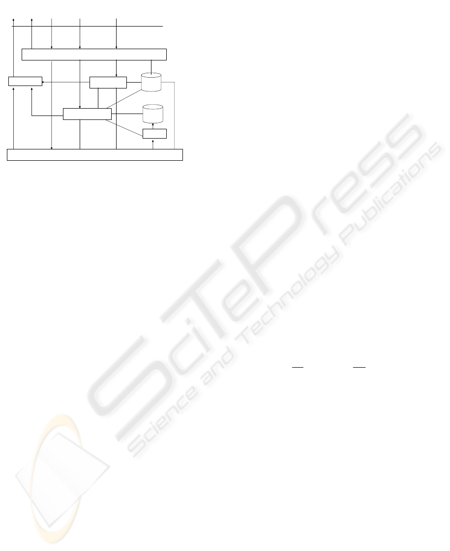
Parser
OLAM
Visualizer
Database API / File System
Loader
OLAP
Metadata
ST trees
SQL CQLError DMQL
Result
GUI API
Figure 2: System architecture that integrates DBMS,
OLAP, and OLAM.
In addition to mining directly on databases or
files, the OLAM engine can also be built on top of
OLAP engines, which is the main topic of this paper.
The OLAP, or data cube server, instructs a loader to
construct ST trees from databases or files so that
later on the cube queries are evaluated using the
initialized ST trees (or SST trees), which is
significantly faster than using DBMS servers
(Hammer and Fu 2001). After the ST tree is
initialized, the data cubes can be extracted from the
leaves to construct decision trees.
5 CONSTRUCTION OF DECISION
TREES USING DATA CUBE
5.1 A General Template of Building
Decision Trees
In decision tree classification, one recursively
partitions the training data set until the records in the
sub-partitions are entirely or mostly from the same
class. When the data cubes have been computed, in
this section we will design a new decision tree
algorithm which builds a tree from data cubes
without accessing original training records any
more.
The internal nodes in a decision tree are called
splits, predicates to specify how to partition the
records. The leaves contain class labels that the
records satisfying the predicates along the root-to-
leaf paths are classified into. We consider binary
decision trees though multi-way trees are also
possible. The following is a general template for
almost all decision tree classification algorithms:
Pa
If (all records in S are of the same
class) then return;
rtition (Dataset S) {
Compute the splits for each
attribute;
Choose the best split to
partition S into S
1
and S
2
;
Partition (S
1
);
Partition (S
2
);
}
An initial call of Partition (training dataset) will
setup a binary decision tree for the training data set.
Before the evaluation of the splits, the domain
values of the training records are all converted into
integers starting from 0. The conversions can be
done during the scanning of original training data.
5.2 Compute the Best Split for the
Root
Given a training dataset with N records each of
which has d predictor attributes and the classifying
attribute B, suppose that they are classified into C
known classes L
p
, p = 0, 1, …, C-1. We use gini-
index to compute the splits at the root of the decision
tree as follows.
|||,|
,
),()()(
||,/)(
,1)(
2211
21
2
2
1
1
1
0
2
SnSn
SandSodpartitioneisSif
Sgini
n
n
Sgini
n
n
Sgini
SnnjBcountp
Sinjclassoffrequencytheispwhere
pSgini
j
j
C
j
j
==
+=
===
−=
∑
−
=
int
A split for continuous attribute A is of form
value(A) ≤ v, where v is the upper bound of some
interval of index k (k = 0, 1, …, V-1, where V is the
total number of values for A). To simplify, let us just
denote this as A ≤ k. The following algorithm
evaluates the best split for attribute A.
1. x[j]=0, for j =0, 1, …, C-1;
CountSum = 0;
2. Gini = minS it = 0; min 1; pl
3. for i = 0 to V-1 do
4. countSumÅcountSum+count(A=i);
5. n
= countSum; n =n-countSum;
1 2
6. squaredSumL, squaredSumH = 0;
7. for j = 0 to C-1 do
8. x[j]=x[j]+count(A=i;B = j);
y = count(B=j) – x[j];
9. sqSumL Å sqSumL+(x[j] /n
1
)
2
;
ICEIS 2005 - ARTIFICIAL INTELLIGENCE AND DECISION SUPPORT SYSTEMS
122

10. sqS
11. endfor
umH Å sqSumH+(y /n
2
)
2
;
12. gini(S
1
)=1-sqSumL;
gini(S
2
)=1- sqSumH;
13. ni(S)=n
gini(S )/n+n (S
2
)/n;
gi
1 1 2
gini
14. if gini(S) < minGini then
15. MiniG
16. endif
ini=gini(S);minSplit = i;
17. endfor
Lines 1 and 2 initialize temporary variables
countSum and array x, and current minimal gini idex
minGini and its split position miniSplit. Lines 3
through 17 evaluate all possible splits A≤ i (i=0, 1,
…, V-1) and choose the best one. Each split
partitions data set S into two subset S
1
= {r in S |
r[A] ≤ i} and S
2
= S-S
1
. Line 4 tries to simplify the
computation of the size of S
1
i.e. count (A ≤ i) by
prefix-sum computation. Similarly, array x[j] is used
to compute count(A ≤ i; B = j) for each class j (j =0,
1, …, C-1) in lines 1 and 8. All these count
expressions are cube queries evaluated by the
method in Sec. 3.
For categorical attributes, the splits are of form
value(A)
∈
T, where T is a subset of all the attribute
values of A. Any such subset is a candidate split.
n
1
= count(value(A)∈ T), and n
2
= n-n
1
p
j
= count(value(A) ∈ T; B = j) / n
1
Knowing how to compute these variables, we can
similarly compute the gini(S) for each split and
choose the best one, as we did for continuous
attributes. The final split for the root is then the split
with the smallest gini index among all the best splits
of the attributes.
5.3 Partitioning and Computing
Splits for Other Internal Nodes
The best split computed above is stored in the root.
All existing decision tree algorithms at this point
partition the data set into subsets according to the
predicates of the split. In contrast, cubeDT does not
move data around. Instead, it just virtually partitions
data by simply passing down the split predicates to
its children without touching or querying the original
data records any more at this phase. The removal of
the expensive process of data partitioning greatly
improves the classification performance.
The computation of splits for an internal node
other than the root is similar to the method in Sec.
5.2 except that the split predicates along the path
from the node to the root are concatenated as part of
constraints in the cube query. For example, suppose
a table containing customer information has three
predictor attributes: age, income, and credit-report
(values are poor, good, and excellent). The records
are classified into two classes: buy or not buy
computer. Suppose the best split of A turns out to be
“age ≤ 30,” and now we are computing splits for the
attribute income at node B. Notice that value n
1
=
count ( income ≤ v; age ≤ 30), and n
2
= count(age ≤
30) – n
1
. Here, we do not actually partition data set
by applying the predicate “age ≤ 30,” instead, we
just form new cube queries to compute the splits for
the node B. As before, these cube queries are
evaluated through partial traversal of ST or SST
trees.
At node C, n
1
= count ( income ≤ v; age > 30),
and n
2
= count(age > 30) – n
1
. All other variables are
computed similarly for evaluating the splits.
Suppose that after computation and comparison the
best split at B is “income ≤ $40, 000,” the diagram
shown in Fig. 3. gives the initial steps of evaluating
splits of nodes A, B, and C.
Age <= 30
Income <= $40K
Yes
No
A
B
C
….
Figure 3: Example of computing splits of non-root internal
nodes.
6 SIMULATIONS
To verify the effectiveness of cubeDT, we have
conducted preliminary studies by comparing it with
BUC (bottom-up cubing) (Beyer and Ramakrishnan
1999) since the predominant time of cubeDT is
spent on the construction of the SST. We compare
with BUC because a family of algorithms such as
BUC, BUC-BST, Condensed Cube, and QC-trees
are all based on recursive partitioning and thus have
similar I/O efficiency. All the experiments are done
on a Dell PC Precision 330, which has a 1.7GHZ
CPU, 256MB memory, and the Windows 2000
operating system. All the algorithms are
implemented in C++.
CONSTRUCTION OF DECISION TREES USING DATA CUBE
123
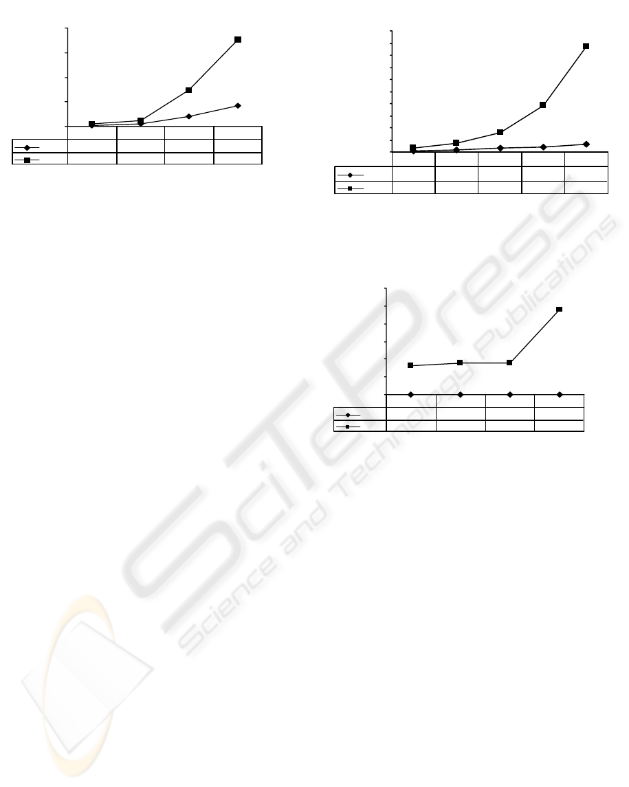
0
500
1000
1500
2000
Number of Records
Runtime (sec.)
SST
22.1 43 209.8 420.46
BUC
50.9 117.9 743.7 1765.3
50K 100K 500K 1M
Figure 4: Varying number of records.
We used uniformly distributed random data and
set each of the five dimensions with a cardinality of
10. The number of records is increased from 50, 000
to 1,000,000 (data set sizes from 1megabytes to 20
megabytes). The runtimes are shown in Fig. 4. SST
is about 2-4 times faster than BUC. The
performance improvements we achieve increase
quickly with an increase in the number of records.
Note that the runtimes are the times for computing
the data cubes.
We also investigate the behaviour of SST and
BUC by varying the number of dimensions and
using data of zipf distribution (factor is 2). We set
the number of records is 100,000 and the cardinality
of each dimension is fixed to 20. The number of
dimensions increases from 4 to 8. Figure 5 shows
the construction times. Clearly SST is scalable with
respect to the number of dimensions.
The query evaluation times are much faster than
construction times. We measure the query times
using total response times of 100 random queries.
The queries are generated by first randomly
choosing three dimensions where random numbers
within the domains are selected as queried values.
All other coordinates in the queries are star values.
Since our SST can fit into memories in these
experiments, queries can be evaluated without I/O’s.
SST is one order faster than other BUC (Figure 6).
0
200
400
600
800
10 0 0
12 0 0
14 0 0
16 0 0
18 0 0
2000
Number of dimensions
Runtime (sec.)
SST
23.8 38.2 58.6 86 122
BUC
61 138 327.5 760.9 1743
45678
Figure 5: Varying number of dimensions.
0
0.5
1
1.5
2
2.5
3
Number of dimensions
Response time (sec.
)
SST
0.01 0.01 0.01 0.01
BUC
0.811 0.881 0.881 2.393
4567
Figure 6: Query response times.
These experiments show that SST has a better
performance, however, notice that cubeDT is
general, i.e. the method of computing data cube is
not restricted to our cubing algorithms using ST or
SST trees. It can be on top of other data cube
systems such as BUC as well.
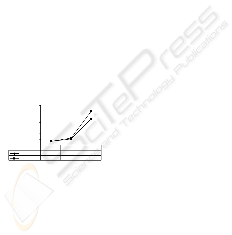
We also compare the performance of cubeDT,
which includes both cube computation and decision
tree generation phases, with that of RainForest
algorithm. According to (Mehta, Agrawal et al.
1996) and (Shafer, Agrawal et al. 1996), SLIQ
produces accurate trees significantly smaller than the
trees produced by IND-C4 (a predecessor of C4.5)
but is almost one order faster than IND-Cart.
SPRINT is faster and more scalable than SLIQ while
producing exactly the same trees as SLIQ. Previous
experiments have also shown that RainForest in
(Gehrke, Ramakrishnan et al. 1998) offers a
performance improvement of a factor five over the
previous fastest algorithm SPRINT. So, we compare
our cubeDT algorithm with RainForest.
Among several implementations of RainForest
such as RF-Read, RF-Write, RF-Hybrid, and RF-
ICEIS 2005 - ARTIFICIAL INTELLIGENCE AND DECISION SUPPORT SYSTEMS
124
Vertical, RF-Read is fastest, assuming that the AVC-
groups of all the nodes at one level of the decision
tree can fit into memory. In this case, one can only
need one scan of reading the input data to compute
the AVC-groups at that level and compute the best
splits from the AVC-groups. Even in this ideal case
(hardly usable in real applications), RainForest
needs at least h passes of original potentially large
input data set, where h is the height of the decision
tree. Other implementations need more read/write
passes. In contrast, cubeDT requires one pass of
input set to compute the cubes, after that, the
decision tree can be built from the data cube without
touching the input data any more. In this set of
experiments, we use uniform data set containing
four descriptive attributes, each of size 10, and the
class attribute has five class values. We increase the
number of records from half million to five millions.
Figure 7 shows that cubeDT is faster, and more
importantly, the performance gap becomes
significantly wider when I/O times become
dominant. The runtimes of cubeDT have already
included the cube generation times, without which
the decision tree construction using cube will be one
order faster than RainForest.
0
2000
4000
6000
8000
10 0 0 0
12 0 0 0
14 0 0 0
Number of Records
Runtime (sec.)
cubeDT
1288 2100 9306
RainForest
1328 2481 12037
500K 1M 5M
Figure 7: Varying number of records.
Since cubeDT uses the same formulas for
computing the splits, it produces the same trees as
SLIQ, SPRINT, and RainForest algorithms, that is,
they have the same accuracy of classification. The
accuracy issue is orthogonal to the performance
issue here. However, cubeDT is significantly faster
due to direct computation of splits from data cube
without actually partitioning and storing the F-sets,
especially when input data sets are so large that the
I/O operations become the bottleneck of
performance.
7 CONCLUSIONS AND FUTURE
WORK
In summary, in this paper we propose a new
classifier that extracts some of the computed data
cubes to setup decision trees for classification. Once
the data cubes are computed by scanning the original
data once and stored in statistics trees, they are ready
to answer OLAP queries. The new classifiers
provide additional “free” classification that may
interest users. Through the combination of
technologies from data cubing and classification
based on decision trees, we pave the way of
integrating data mining systems and data cube
systems seamlessly. An architecture design of such
an integrated system has been proposed. We will
continue the research on the design of other efficient
data mining algorithms on data cube in the future.
REFERENCES
Agarwal, S., R. Agrawal, et al. (1996). On The
Computation of Multidimensional Aggregates.
Proceedings of the International Conference on Very
Large Databases, Mumbai (Bomabi), India: 506-521.
Beyer, K. and R. Ramakrishnan (1999). Bottom-Up
Computation of Sparse and Iceberg CUBEs.
Proceedings of the 1999 ACM SIGMOD International
Conference on Management of Data (SIGMOD '99).
C. Faloutsos. Philadelphia, PA: 359-370.
Chan, C. Y. and Y. E. Ioannidis (1998). Bitmap Index
Design and Evaluation. Proceedings of the 1998 ACM
SIGMOD International Conference on Management of
Data (SIGMOD '98), Seattle, WA: 355-366.
Chaudhuri, S. and U. Dayal (1997). "An Overview of Data
Warehousing and OLAP Technology." SIGMOD
Record 26(1): 65-74.
Chaudhuri, S., U. Fayyad, et al. (1999). Scalable
Classification over SQL Databases. 15th International
Conference on Data Engineering, March 23 - 26,
1999, Sydney, Australia: 470.
Cheeseman, P. and J. Stutz (1996). Bayesian
Classification (AutoClass): Theory and Results.
Advances in Knowledge Discovery and Data Mining.
R. Uthurusamy, AAAI/MIT Press: 153-180.
Comer, D. (1979). "The Ubiquitous Btree." ACM
Computing Surveys 11(2): 121-137.
Duda, R. and P. Hart (1973). Pattern Classification and
Scene Analysis. New York, John Wiley & Sons.
Fu, L. (2003). Classification for Free. International
Conference on Internet Computing 2003 (IC'03) June
23 - 26, 2003, Monte Carlo Resort, Las Vegas,
Nevada, USA.
CONSTRUCTION OF DECISION TREES USING DATA CUBE
125

Fu, L. and J. Hammer (2000). CUBIST: A New Algorithm
For Improving the Performance of Ad-hoc OLAP
Queries. ACM Third International Workshop on Data
Warehousing and OLAP, Washington, D.C, USA,
November: 72-79.
Gehrke, J., V. Ganti, et al. (1999). BOAT - Optimistic
Decision Tree Construction. Proc. 1999 Int. Conf.
Management of Data (SIGMOD '99), Philadephia,
PA, June 1999.: 169-180.
Gehrke, J., R. Ramakrishnan, et al. (1998). RainForest - A
Framework for Fast Decision Tree Construction of
Large Datasets. Proceedings of the 24th VLDB
Conference (VLDB '98), New York, USA, 1998: 416-
427.
Hammer, J. and L. Fu (2001). Improving the Performance
of OLAP Queries Using Families of Statistics Trees.
3rd International Conference on Data Warehousing
and Knowledge Discovery DaWaK 01, September,
2001, Munich, Germany: 274-283.
Han, J. and M. Kamber (2001). Data Mining: Concepts
and Techniques, Morgan Kaufman Publishers.
Harinarayan, V., A. Rajaraman, et al. (1996).
"Implementing data cubes efficiently." SIGMOD
Record 25(2): 205-216.
Inmon, W. H. (1996). Building the Data Warehouse. New
York, John Wiley & Sons.
Johnson, T. and D. Shasha (1997). "Some Approaches to
Index Design for Cube Forests." Bulletin of the
Technical Committee on Data Engineering, IEEE
Computer Society 20(1): 27-35.
Lakshmanan, L. V. S., J. Pei, et al. (2003). QC-Trees: An
Efficient Summary Structure for Semantic OLAP.
Proceedings of the 2003 ACM SIGMOD International
Conference on Management of Data, San Diego,
California, USA, June 9-12, 2003. A. Doan, ACM:
64-75.
Lent, B., A. Swami, et al. (1997). Clustering Association
Rules. Proceedings of the Thirteenth International
Conference on Database Engineering (ICDE '97),
Birmingham, U.K.: 220-231.
Lu, H., R. Setiono, et al. (1995). NeuroRule: A
Connectionist Approach to Data Mining. VLDB'95,
Proceedings of 21th International Conference on Very
Large Data Bases, September 11-15, 1995, Zurich,
Switzerland. S. Nishio, Morgan Kaufmann: 478-489.
Mehta, M., R. Agrawal, et al. (1996). SLIQ: A Fast
Scalable Classifier for Data Mining. Advances in
Database Technology - EDBT'96, 5th International
Conference on Extending Database Technology,
Avignon, France, March 25-29, 1996, Proceedings. G.
Gardarin, Springer. 1057: 18-32.
O'Neil, P. (1987). Model 204 Architecture and
Performance. Proc. of the 2nd International Workshop
on High Performance Transaction Systems, Asilomar,
CA: 40-59.
O'Neil, P. and D. Quass (1997). "Improved Query
Performance with Variant Indexes." SIGMOD Record
(ACM Special Interest Group on Management of
Data)
26(2): 38-49.
Quilan, J. R. (1986). Introduction of Decision Trees.
Machine Learning. 1: 81-106.
Quilan, J. R. (1993). C4.5: Programs for Machine
Learning, Morgan Kaufmann.
Shafer, J., R. Agrawal, et al. (1996). SPRINT: A Scalable
Parallel Classifier for Data Mining. VLDB'96,
Proceedings of 22th International Conference on Very
Large Data Bases, September 3-6, 1996, Mumbai
(Bombay), India. N. L. Sarda, Morgan Kaufmann:
544-555.
Sismanis, Y., A. Deligiannakis, et al. (2002). Dwarf:
shrinking the PetaCube. Proceedings of the 2002 ACM
SIGMOD international conference on Management of
data (SIGMOD '02), Madison, Wisconsin: 464 - 475.
Zhao, Y., P. M. Deshpande, et al. (1997). "An Array-
Based Algorithm for Simultaneous Multidimensional
Aggregates." SIGMOD Record 26(2): 159-170.
ICEIS 2005 - ARTIFICIAL INTELLIGENCE AND DECISION SUPPORT SYSTEMS
126
