
THE ROBUSTNESS OF BLOCKING PROBABILITY IN A LOSS
SYSTEM WITH REPEATED CUSTOMERS
Akira Takahashi, Yoshitaka Takahashi
Graduate School of Commerce , Waseda University
Shinjuku, Tokyo 169-8050, Japan
Shigeru Kaneda, Yoshikazu Akinaga and Noriteru Shinagawa
Network Laboratories , NTT DoCoMo,Inc.
3-5, Hikarinooka, Yokosuka, Kanagawa, 239-8536, Japan
Keywords:
Teletraffic analysis, loss system, repeated customers, Little’s formula.
Abstract:
In this paper, we analyze and synthesize a multi-server loss system with repeated customers, arising out of NTT
DoCoMo-developed telecommunication networks. We first provide the numerical solution for a Markovian
model with exponential retrial intervals. Applying Little’s formula, we derive the main system performance
measures (blocking probability and mean waiting time) for general non-Markovian models. We compare the
numerical and simulated results for the Markovian model, in order to check the accuracy of the simulations.
Via performing extensive simulations for non-Markovian (non-exponential retrial intervals) models, we find
robustness in the blocking probability and the mean waiting time, that is, the performance measures are
shown to be insensitive to the retrial intervals distribution except for the mean.
1 INTRODUCTION
When the service system becomes extremely con-
gested, a lot of customers cannot receive immediate
service. Some of them may give up the service to
leave the system, while others may stay in the sys-
tem and retry their requests. This behavior of re-
peated customers leads to an additional load on the
system and worsens its congestion. The importance
of repeated requests on the performance of the ser-
vice system was pointed out in the late 1940, and
many researches have been performed since then. Pi-
oneering studies on the multi-server loss system with
repeated calls brought some kind of positive expres-
sions of performance measures (See (Falin and Tem-
pleton, 1997), (Artalejo and Pozo, 2002), and (Uda-
gawa and Miwa, 1965)). However, they are not neces-
sarily convenient to calculate performance measures.
Retrial queuing models including one discussed here
are usually very complicated for queuing analysis and
its results are not always suitable to numerical calcu-
lation. Many authors reported numerical approaches
of approximation and truncation methods. For details
on the numerical approaches, readers are referred to
(Artalejo and Pozo, 2002) and (Stepanov, 1999).
Most of them assume that the time intervals be-
tween repeated attempts are mutually independent
and exponentially distributed. However, affected by
many factors and circumstances, customers’ behav-
ior in repeating is so complex that these assumptions
may lead to a risky assessment. There is necessity for
generalization of the retrial interval distribution.
This assumption of exponential retrial intervals is
a kind of simplification for queuing analysis. There
is no guarantee that repeating customers behave in
such a manner. Under this assumption, the number
of repeated requests emerging in a unit time changes
by the state of the retrial queue (See (Artalejo et al.,
2001)). There is another type of retrial queuing model
in which retrial rate is constant. In this type of model,
blocked customers who want to repeat must wait in
line and only the customer at the head of the line can
retry to hunt, if any, an idle server. It has a wide
range of applications like communication protocols.
However, still there are systems more appropriately
modeled by the classical type. On the constant re-
trial policy, there are fruitful investigations of mod-
els with single-server non-exponential retrial intervals
like (G
´
omez-Correl and Ramalhoto, 1999). However,
it remains open problem to investigate the effect of
the retrial times distribution on the performance of the
system. Customers’ behavior in repeating is expected
to be highly complex and it may be risky or ineffi-
cient to build and operate the system upon the results
of exponential assumption. Thus, one finds it neces-
sary to study sensitivity and robustness of the retrial
60
Takahashi A., Takahashi Y., Keneda S. and Akinaga Y. (2005).
THE ROBUSTNESS OF BLOCKING PROBABILITY IN A LOSS SYSTEM WITH REPEATED CUSTOMERS.
In Proceedings of the Second International Conference on e-Business and Telecommunication Networks, pages 61-66
DOI: 10.5220/0001416300610066
Copyright
c
SciTePress

time distribution
The main goal of this paper is to investigate the ro-
bustness (insensitivity) property between the perfor-
mance measure and the retrial time distribution in a
loss system with repeated customers seen in an NTT
DoCoMo developed telecommunication network.
The rest of the paper is organized as follows. Sec-
tion 2 gives teletraffic analysis of the retrial model.
The main performance measures of practical inter-
est are then derived. In Section 3, simulation results
of non-exponential (deterministic/ two-stage Erlang/
two-stage hyper-exponential) retrial models are com-
pared to find robustness of the system.
2 NUMERICAL RESULTS
2.1 Model Description
Consider the following loss system with repeated
calls : (1) There are c servers in parallel; (2) Cus-
tomers’ service times, which are identical and inde-
pendent from one another, are exponentially distrib-
uted with rate µ; (3) Customer arrivals follow a Pois-
son process of rate λ; (4) Customers who find all sev-
ers busy at their arrival epoch choose either to repeat
their requests with probability p or to give up the ser-
vice with probability (1−p); (5) When they decide to
repeat, customers wait in the retrial queue for a ran-
dom time called ”retrial interval”, which is exponen-
tially (generally) distributed with parameter γ in Sec-
tion 2.2( Section 3) before making repeated requests;
(6) Retrial customers who find again all servers busy
choose either to waint in the retrial queue and repeat
their requests with probability p or to stop repeating
and leave the system with probability (1 − p); (7)
Give-up customers leave the system immediately.
We introduce following notations. Suppose the ex-
istence of the stationary state, the state of the sys-
tem is characterized by (1) the number of the busy
servers and (2) the number of the customers waiting
to make a repeated attempt. The system will be said
to be in state (i, j) , if i servers busy and j customers
waiting to repeat. If there are c servers in the sys-
tem then the system is somewhere in the state space
{0, 1, ··· , c} ×{0, 1, ···} . Let π
i,j
denote the prob-
ability that the system is in state (i, j) from now on.
2.2 Calculation of the Stationary
Distribution
By focusing on the possible state transition in a
minute time ∆t, we get the state-transition probabili-
ties as shown in Table 1. Figure 1 illustrates the state-
transition diagram of this model.
Table 1: State-transition probabilities
state-transition probability
(i + 1, j)
↑ (0 ≦ i ≦ c − 1, 0 ≦ j) λ∆t + o(∆t)
(i, j)
(i + 1, j − 1)
տ (0 ≦ i ≦ c − 1, 1 ≦ j) jγ∆t + o(∆t)
(i, j)
(i, j)
↓ (1 ≦ i ≦ c, 0 ≦ j) iµ∆t + o(∆t)
(i − 1, j)
(c, j) → (c, j + 1)
λα∆t + o(∆t)
(0 ≦ j)
(c, j − 1) ← (c, j)
jγ(1 − α)∆t
(1 ≦ j) +o(∆t)
(c, j − 1) ← (c, j)
jγ(1 − α)∆t
(1 ≦ j) +o(∆t)
By Table 1, the state-equilibrium equations are ex-
pressed as below.
(λ + jγ)π
0,j
= µπ
1,j
.
(λ + iµ + jγ)π
i,j
= λπ
i−1,j
+ (j + 1)γπ
i−1,j
+ (i + 1)µπ
i+1,j
(1 ≦ i ≦ c − 1).
(λα + cµ + jγ(1 −α))π
c,j
.
= λπ
c−1,j
+ γπ
c−1,j
+ λαπ
c,j−1
+ (j + 1)γ(1 − α)π
c,j+1
.
Our research purpose here is to study the effect
of the retrial interval distribution and the existence
THE ROBUSTNESS OF BLOCKING PROBABILITY IN A LOSS SYSTEM WITH REPEATED CUSTOMERS
61
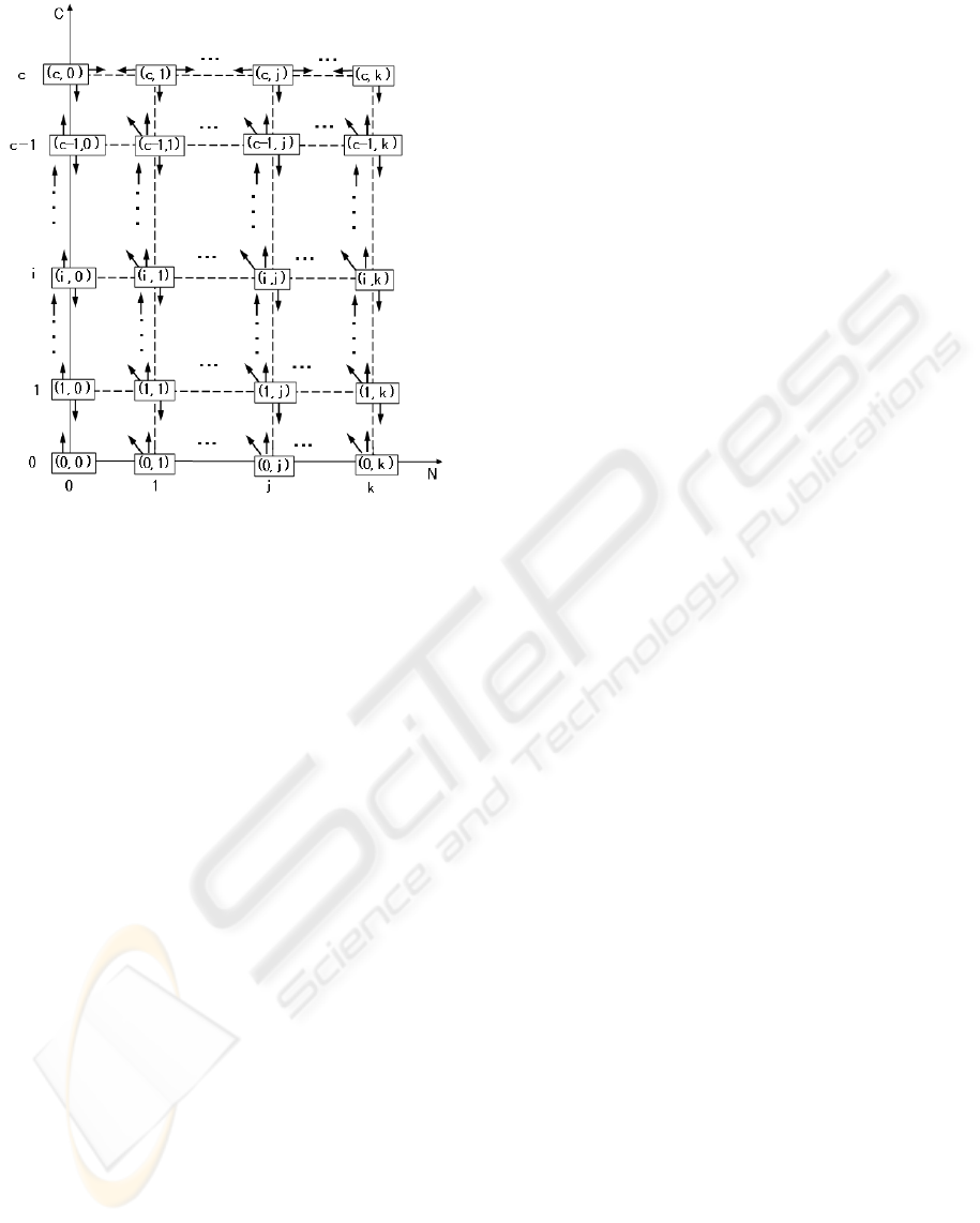
Figure 1: State-transition diagram.
of robustness. To this end, we adopt an simple ap-
proximation method of replacing the infinite space for
customers waiting to repeat requests by a finite num-
ber k. It is an extension of the way to calculate the
steady-state probabilities introduced in (Hashida and
Kawashima, 1979) and closely explained in (Falin
and Templeton, 1997), so we only show the outline of
the algorithm. Here, k is assumed to be a sufficiently
large positive integer so that the overflow probability
is small enough to be ignored. From a finite capacity
argument,
for 1 ≦ j ≦ k − 1,
(λ + jγ)π
0,j
= µπ
1,j
, (1)
(λ + iµ + jγ)π
i,j
= λπ
i−1,j
+(j + 1)γπ
i−1,j
+ (i + 1)µπ
i+1,j
(1 ≦ i ≦ c − 1), (2)
(λα + cµ + jγ(1 −α))π
c,j
= λπ
c−1,j
+ γπ
c−1,j
+ λαπ
c,j−1
+(j + 1)γ(1 − α)π
c,j+1
. (3)
For j = k,
(λ + kγ)π
0,k
= µπ
1,k
, (4)
(λ + iµ + kγ)π
i,k
= λπ
i−1,k
+ (i + 1)µπ
i+1,k
(1 ≦ i ≦ c − 1), (5)
(cµ + kγ(1 − α))π
c,k
= λπ
c−1,k
+ λαπ
c,k−1
. (6)
These recurrence equations enable us to compute
the stationary distribution via the following steps.
(I) Take the appropriate k and introduce auxiliary
variables φ
i,j
, pi
i,j
/π
0,k
.
(II) By definition , φ
0,k
= 1.
From (4), φ
1,k
can be determined.
From (5), one can get φ
i,k
(i = 2, 3, ··· , c)
sequentially.
(III) Equations (1) and (2) for i = 1, ··· , c − 1
constitute a set of c equations with c + 1
unknown variables φ
0,k
, φ
1,k
, ··· , φ
c−1,k
, φ
c,k
. Thus, with φ
c,k
obtained by (6), one
finds the set of equations become solvable .
Hence, (3) gives φ
c,k−2
D
(IV ) Operating steps (I), (II), and (III)
repeatedlyC we get all of the φ
i,j
.
The normalization condition;
P
c
i=0
P
k
j=0
φ
i,j
= 1/φ
0,k
settles π
0,k
and φ
i,j
× π
0,k
gives π
i,j
.
(V ) By repeating from (I) to (IV ) with k plus 1
until the value of π
c,k
becomes less than 10
−10
,
π
i,j
can be calculated with an accuracy enough
for our purpose.
2.3 Performance Measures
We are now in a position to derive the performance
measures of the system.
Time congestion (B
T
)
Letting B
T
be the time congestion, so called, the
probabilities that all the servers are busy, we have
B
T
=
k
X
j=0
π
c,j
.
Blocking probability (B)
When they blocked due to all servers busy, customers
can wait for some random time and retry. After sev-
eral retrials, some of them may give up the service
demand, and leave the system. Here, we define the
ICETE 2005 - WIRELESS COMMUNICATION SYSTEMS AND NETWORKS
62

blocking probability B as the probability that cus-
tomers finally leave without getting served due to suc-
cessive blockings.
To the best of authors’ knowledge, there are few in-
vestigations for a general retrial model. Here, apply-
ing Little’s formula (Little, 1961) enables us to prove
the following proposition.
Proposition 1 Consider a general retrial queuing
system which has input with rate λ, service with rate
µ and retrial with rate γ. Customers who try to re-
ceive a service and get blocked due to all servers busy,
choose either to repeat their requests with probability
p or to stop repeating and leave the system with prob-
ability (1 − p). Blocking probability B, that is, the
probability that arriving customers finally leave the
system with not receiving the service, is expressed by
B = 1 −
1
ρ
C.
Here, ρ denotes traffic intensity defined by λ/µ and
C stands for the mean number of busy servers on the
stationary condition. See Appendix 1 for the proof.
It should be noted that Proposition 1 has a different
expression on the blocking probability from that in
(Hashida and Kawashima, 1979), where the P AST A
(P oisson Arrivals See T ime Averages) property
is heuristically used to provide an approximation. Our
expression on the loss probability shown in Proposi-
tion 1 is exact (not approximate).
Mean waiting time (W q)
Denote by Wq the mean waiting time, namely, the
mean elapsed time from a customer’s arrival epoch
until the epoch where the customer gets served or
stops repeating without receiving its service to leave
the system.
Like B above, W q is also derived from Little’s for-
mula and its relation to other parameters is preserved
under more general situation. So we find the follow-
ing proposition.
Proposition 2 Consider a general retrial queuing
system which has input with rate λ, service with rate
µ and retrial with rate γ. Customers who try to re-
ceive a service and get blocked due to all servers busy,
choose either to repeat their requests with probability
p or to stop repeating and leave the system with prob-
ability (1 − p). The mean waiting time W q, that is,
the time that customers have to spend on average until
they finally get served or decide to stop repeating and
leave, is expressed by
W q =
K
λ
.
K is the mean number of customers in the retrial area
in the steady state. See Appendix 2 for the proof.
3 SIMULATION RESULTS
In the previous section, we get the numerical solution
of the loss system with exponential retrial intervals.
Next, we change the assumption about retrial. In this
section we compare performance measures between
the exponential retrial interval model and the mod-
els with non-exponential retrial intervals. Even un-
der the exponential retrial interval assumption, multi-
server property involves great complicity and analyt-
ical solutions are obtained only a few special cases
like (Falin and Templeton, 1997) and (Choi and Kim,
1998). So we employ computer simulation to esti-
mate the performance measure of non-exponential re-
trial interval models. The assumptions for simulation
are all the same with those for numerical calculation
introduced in Section 2 except for the distribution of
retrial intervals. It assumes a Poisson arrival of cus-
tomers with rate λ and an identically independently
distributed exponential service time with rate µ.
On the distribution of retrial intervals, in this pa-
per we take four different models; the exponential re-
trial interval model (Exp model) the constant retrial
interval model (D model), the 2-stage Erlang distrib-
ution model (E2 model), and the 2-stage hyper expo-
nential distribution model (H2 model). Among H2
models, we also have three different types whose co-
efficient of variation (C
X
) of the retrial interval dis-
tribution is lager than 1, equal to 1, or smaller than
1. In other words, the variance of the retrial in-
terval distribution is large, equal or small in com-
parison to its mean. H2(C
X
=
√
2), H2(C
X
=
√
20) and H2(C
X
=
√
200) denote the model with
hyper-exponential retrial intervals whose C
X
equals
to
√
2,
√
20 and
√
200, respectively .
Through this section, τ , µ/γ is used for the indi-
cator of the mean retrial interval and ρ , λ/µ for the
traffic offered to the whole system.
In simulation, c(= the number of servers) is set to
10, µ 0.01and p 5/6, which means the service time
average is 100 and under the condition of successive
blocking customers continue to repeat 5 times on av-
erage. An individual simulation results (expressed as
points in each figure) is based on 50 runs(approx. 5
hours on IBM Thnkpad PC).
First, the accuracy of the simulation should be in-
vestigated. Figure 2 shows the blocking probability
B by numerical calculation and simulation with the
mean retrial time τ = 1. As seen in Figure 2, we can-
not see significant difference between our numerical
and simulation results. Therefore, our simulation re-
sults are very accurate. The accuracy of simulation is
confirmed on other performance measures.
Now that we see the accuracy of the simulation,
comparisons are performed when the mean retrial in-
terval τ is 0.01, 1, and 100.0, which corresponds to
THE ROBUSTNESS OF BLOCKING PROBABILITY IN A LOSS SYSTEM WITH REPEATED CUSTOMERS
63
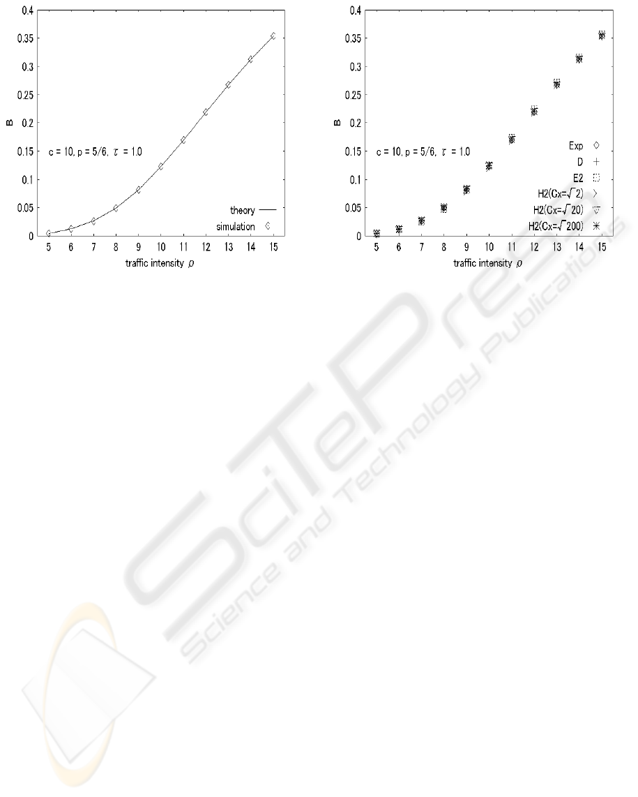
Figure 2: The blocking probability B by numeric al
calculation and simulation.
the situations that repeated requests arises 100 times
sooner than the service time on average, that they
arise with the interval as long as the service time on
average, and that they arise after a time 100 times
longer than the service time on average.
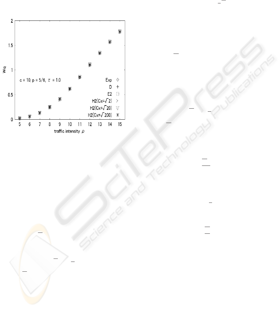
Figures 3 and 4 show the relationship of the block-
ing probability B and the mean waiting time W q to
the traffic intensity ρ. One finds the retrial interval
distribution makes little difference.
4 CONCLUSION
We have analyzed and synthesized a multi-server
loss system with repeated customers, arising out
of NTT DoCoMo-developed telecommunication net-
works. We have first provided the numerical solution
for a Markovian model with exponential retrial in-
tervals. Applying Little’s formula, we have derived
the main system performance measures (blocking
probability and mean waiting time) for general non-
Markovian models. We have compared the numeri-
cal and simulated results for the Markovian model, in
order to check the accuracy of the simulations. Via
performing extensive simulations for non-Markovian
(non-exponential retrial intervals) models, we have
found robustness in the blocking probability and the
mean waiting time, that is, the performance measures
have been shown to be insensitive to the retrial inter-
vals distribution except for the mean.
It is left for future work to investigate the robust-
ness for a more general (e.g., a general service time
distribution) model.
Figure 3: The blocking probability B versus the traffic
intensity ρ.
ACKNOWLEDGEMENT
The present research was partially supported by a
Grant-in-Aid for Scientific Research (C) from Japan
Society for the Promotion of Science under Grant No.
1458049.
REFERENCES
Artalejo, J., G
´
omez-Correl, A., and Neuts, M. (2001).
Analysis of multiserver queues with constant retrial
rate. European Journal of Operational Research,
135:569–581.
Artalejo, J. and Pozo, M. (2002). Numerical calculation
of the stationary distribution of the main multiserver
retrial queue. Annals of Operations Research, 116:41–
56.
Choi, B. and Kim, Y. (1998). The M/M/c retrial queue with
geometric loss and feedback. Computers and Mathe-
matics with Applications, 36:41–52.
Falin, G. and Templeton, J. (1997). Retrial Queues. Chap-
man and Hall, London, 1st edition.
G
´
omez-Correl, A. and Ramalhoto, M. (1999). The station-
ary distribution of a markovian process arising in the
theory of multiserver retrial queueing systems. Math-
ematical and Computer Modelling, 30:141–158.
Hashida, O. and Kawashima, K. (1979). Buffer behav-
ior with repeated calls. The IECE Transactions, J62-
B:222–228.
Little, J. D. C. (1961). A proof for the queuing formula: L =
λ W. The Journal of the Operations Research Society
of America, 9:383–387.
ICETE 2005 - WIRELESS COMMUNICATION SYSTEMS AND NETWORKS
64
Stepanov, S. (1999). Markov model with retrials:the cal-
culation of stationary performance measures based on
the concept of truncation. Mathematical and Com-
puter Modelling, 30:207–228.
Udagawa, K. and Miwa, E. (1965). A complete group of
trunks and poisson-type repeated calls which influ-
ence it. The IECE Transactions, 48:1666–1675.
Figure 4: The mean waiting time W q versus the traffic
intensity ρ.
APPENDICES
Appendix 1
Proof of Proposition 1
We restrict ourselves to the sub-system only composed
of c servers. We apply Little’s formula [ L = λW ] (Little,
1961) to this sub-system.
Let λ
′
and
C respectively denote the sub-system
throughput and the mean number of busy servers. By Lit-
tle’s formula, we have
C = λ
′
1
µ
, (A.1)
now that
C [the mean number of customers in the sub-
sytem] corresponds to L, λ
′
[the effective arrival rate of the
sub-system] corresponds to λ, and 1/µ [the mean sojourn
time in the sub-system] corresponds to W .
The blocking probability B is defined as the probabil-
ity that an arriving customer cannot finally receive its ser-
vice, however often it may repeat the retrial process [being
blocked, waiting, and retrying].
Since on average λ customers arrive at the system in unit
time, the mean number of customers who leave the system
without being served is given by λB. The mean number of
customers who receive their services is obtained as
λ(1 − B) = λ
′
. (A.2)
Substituting (A.2) into (A.1), and solving for B we fi-
nally get
B = 1 −
1
ρ
C.
Appendix 2
Proof of Proposition 2
We restrict ourselves to the sub-system only composed
of the retrail queue (with a finite capacity of k customers).
We apply Little’s formula [ L = λW ] to this sub-system.
Let S and
K denote the mean number of retrials and the
mean number of customers in the retrial queue, respectively.
Since on average λ customers arrive at the system in time
unit, then each one of them go through the retrial queue S
times on average. That is, the mean number of customers
who go to the retrial queue in time unit equals to Sλ. By
Little’s formula, we have
K =Sλ
1
µ
(A.3)
now that
K [the mean number of customers in the sub-
sytem] corresponds to L, Sλ [the effective arrival rate of the
sub-system] corresponds to λ, and 1/µ [the mean sojourn
time in the sub-system] corresponds to W . From (A.3), we
have
S =
Kγ
λ
(A.4)
Since the mean retrial interval is 1/µ and customers re-
peat their requests S times on average, then the mean waint-
ing time W q is
W q = S
1
γ
(A.5)
Substituting (A.4) to (A.5), we get
W q =
K
λ
.
THE ROBUSTNESS OF BLOCKING PROBABILITY IN A LOSS SYSTEM WITH REPEATED CUSTOMERS
65
