
Comparison of Time and Spectral Domain Features on
Postural Signals Utilizing Neural Networks
Andreas Fey, David Sommer, Martin Golz
FH Schmalkalden - University of Applied Sciences, Dptm. of CS,
Postfach 10 04 52, 98574 Schmalkalden, Germany
Abstract. Human postural equilibrium is the result of complex control
processes. Nevertheless these processes are taken for granted in our daily life,
disturbance or degeneration of a single system involved in these processes leads
to a variety of diseases, which pile up with age. Therefore, investigation of
postural signals is the aim of many clinical and biophysical studies, in order to
recognize diseases early and to improve the precision of diagnostics. In order to
analyze posturographic signals we conducted a pilot study to measure body
sway of nine healthy subjects during four trials with different acoustic and
visual impairments, in order to detect their influence on stance. Ten time
domain and five spectral domain feature extraction methods were applied on
segmented raw data and classified by five different classification methods. The
test errors were empirically minimized first by estimating best parameters for
each feature extraction method, yielding to an optimal combination of feature
extraction and classification methods. It turned out, that Burg autoregressive
method of power spectral density estimation and Optimized Learning Vector
Quantization was the best method combination. The classification task “no
impairment” versus “visual impairment”, i.e. “eyes open” versus “eyes closed”,
showed best discriminative performance indicated by mean test errors of 2.2%.
The pilot study pointed out, that the established biosignal analysis system
gained a high sensitivity on small postural influences.
1 Introduction
During erect standing several muscles are permanently contracted in order to stabilize
body sway and prevent the body from falling. The control mechanisms in the central
nervous system for these muscles are influenced by a multisensory input, subdivided
in the vestibular, proprioceptive and visual system [3]. Disturbances or degenerations
of only one of these systems lead to a variety of diseases, including falls, Ménière’s
disease, cerebellar degeneration or uni- and bilateral vestibular malfunction. The
annual costs associated with falls are exceeded only by motor vehicle injuries [11].
Many clinical and biophysical studies aimed therefore the investigation of postural
signals for early recognition of diseases and a more precise diagnostic. In order to
examine different states of equilibrium, usually a single system is stimulated or
disabled, e.g. the visual system by closing both eyes, the proprioceptive system by
Fey A., Sommer D. and Golz M. (2005).
Comparison of Time and Spectral Domain Features on Postural Signals Utilizing Neural Networks.
In Proceedings of the 1st International Workshop on Biosignal Processing and Classification, pages 42-49
DOI: 10.5220/0001196100420049
Copyright
c
SciTePress

adding vibratory stimuli at the calf muscles or the vestibular system by applying tones
at the ear.
Auditory stimuli is a wide spread method to provoke the vestibular system, and is
used for this reason since the 30s. The mechanisms underlying this effect are not fully
understood. Some authors assume sound giving rise to contractions of middle-ear
muscles resulting in excessive jerking of the stapes and causing movements of the
perilymph in semicircular canal system [14]. In the 80s and 90s some studies
examined the influence of various frequencies and loudness on postural sway, and
showed that varying frequencies have a primary effect on antero-posterior sway,
while changing the loudness results in medio-lateral sway. Different frequencies seem
to have a stabilizing or destabilizing effect as well [17]. Another variation in acoustic
stimulation beside frequency and loudness is the continuity of the tones. Even in 1929
Thullio showed, that tones intended on only one ear provoke symptoms like sway or
nystagmus, while binaural stimulations preserve this effect. Interrupted tones
additionally increase this effect [6]. At least the direction of the tones was also
examined resulting in greater effects of moving auditory stimuli compared to
stationary auditory stimuli [17][16].
In order to estimate the sensitivity of postural sway measures on small and on
serious influences we conducted a pilot study including nine healthy subjects. As an
example of serious influences we selected visual impairments by occluding the eyes
and therefore interrupting visual feedback. Binaural presented moving acoustic
stimuli served as small influences.
Based on a literature inquiry of the last decade, ten important time domain and five
spectral domain feature extraction methods were established. Performance analysis
utilizing Neural Networks was carried out.
2 Methods
Postural sway of nine healthy volunteers without known visual, proprioceptive or
vestibular diseases was measured in four trials of different modalities with / without
interruption of visual feedback (00 / 10) and with / without binaural stimulation (00 /
01 / 02):
1. eyes open, normally illuminated environment, no auditive stimuli (00)
2. eyes closed and occluded , fully darkened environment, no auditive stimuli (10)
3. eyes closed and occluded, fully darkened environment, periodic randomized noise
from left to right ear of one second length (11)
4. eyes closed and occluded, fully darkened environment, periodic randomized noise
from left to right ear of 2.5 second length (12)
Symbol “0” stands for no impairment, while symbol “1” and “2” stand for
impairment. The first symbol concerns visual, the second acoustic impairments. Each
trial of 100 second duration was followed by a recovery time of one minute and
additionally by one minute for darkness adaption after the first trial.
Recordings of postural sway were performed on a force platform on which subjects
had to stand upright. Signals of four force sensors located under the platform were
sampled with a rate of 1000 sec
-1
and were subsequently processed to calculate two
43
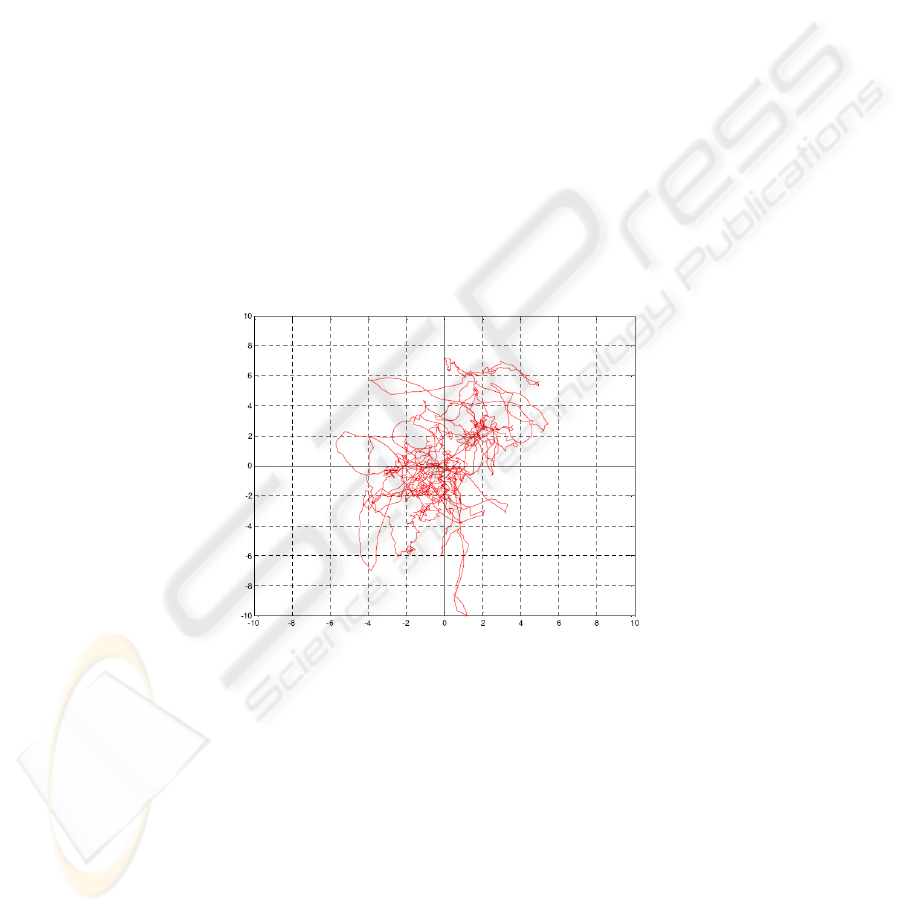
dimensional vectors of locations of the center-of-foot-pressure (COP). The time series
of COP visualized in medio-lateral and antero-posterior direction as y- and x-axis
respectively is called stabilogram (figure °1).
Because the classification methods used here require lots of data for learning to
raise the generalization effect, although stationarity of the signal is required for
following methods, we segmented the raw data and estimated the optimal segment
length empirically. While a short segment length would raise the quantity of data,
long segments would improve the spectral resolution and therefore improve the
quality of results of the spectral domain features.
15 different feature extraction methods (table °1) of time and spectral domain
which were commonly used by several authors in the last two decades were applied
than to the segmented data. Spectral power density (PSD) was computed by spectral
domain features. Subsequently PSDs were averaged in frequency bands because of
the resulting large amounts of components and because of their high variances, which
are typical for biomedical signals as realizations of random processes. The adjustable
parameters for the spectral domain feature extraction methods are therefore lower and
upper cut-off frequency f
L
and f
U
respectively and the band width ∆f. The range
between f
L
and f
U
is equidistant divided with step size ∆f. For Burg and MTM
additionally another parameter (model order / time-bandwidth product [15]) was
empirically computed. Band averaged PSDs were then used as components of input
vectors for all classification methods.
Fig. 1. Stabilogram of one subject. Time series of medio-lateral (x) and anterior-posterior (y)
components of Centre-of-Pressure measured in upright standing with opened eyes; duration:
100 sec, sampling rate: 1,000 sec
-1
All ten time-domain methods plus the total spectral energy resulted in 23 different
features. Because each feature would be to less data for the classification methods, all
of them were combinated to a 23 dimensional input vector. Each possible
combination (2²³ combinations = 8.388.608 possibilities) was applied to the
classification methods to evaluate the best classifiable input vector of time domain
features empirically.
x
n
[mm]
y
n
[mm]
44

Table 1. Utilized feature extraction methods in time and spectral domain with references to
authors using this methods in the last decade
Time domain Spectral domain
Sway path [17] [12] [1] Sway area [17] [12] [1] Periodogram (PSD) [15]
Root mean squares [1] Amplitudes of COP [17] Welch Overlapped Segments
Analysis (PSD) [15]
Mean [17] Maximal displacement [17] Burg autoregressive method
(PSD) [15]
Standard deviation [17] Stabilogram diffusion plot
[1]
Multitaper Method (PSD) [15]
Sway velocity [17] Sway density curve [2] Total spectral energy [12] [1]
The test error was computed using the leave-one-out (LOO) cross-validation. LOO
estimates this error by removing sequentially one sample from the training samples,
using the remaining samples for training and leading to a classification rule, which is
tested on the held-out example [7]. LOO leads to a high computational cost (n-1
repetitions for n samples), but is an almost unbiased estimator of the true error.
At least we compared the following classification methods empirically by taking
test errors estimated by LOO into account:
1. Learning Vector quantization (LVQ), with variants [8]
2. Self Organizing Maps (SOM) [9]
3. Growing Cell Structures (GCS) [5]
4. Support Vector Machine (SVM) [18]
3 Results
3.1 Parameter optimization by empirical error minimization
The following examinations were carried out to find optimal parameters in all steps of
the classification process and therefore minimize the empirical error. OLVQ
classification method was used because of its fast convergence properties. 00 vs. 10,
the typical “eyes open” versus “eyes closed” combination, examined by most authors
(eg. [2], [4]) in posturographic studies, was tested.
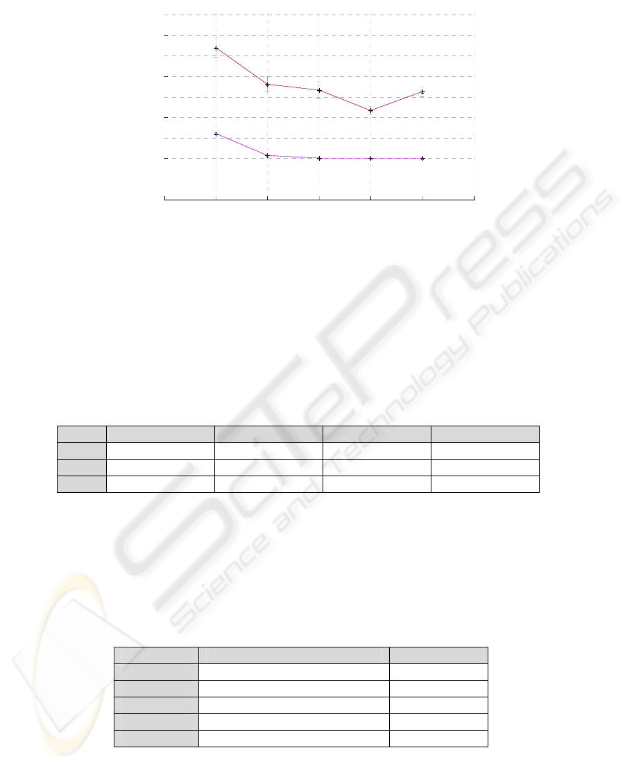
For estimation of the optimal segment length, we empirically tested several lengths
from 5 to 25 seconds with steps of 5 seconds. A length of 20 seconds showed the best
results, leading to 5 times of the amount of data in contrast to the raw data (figure °2).
In order to estimate the best frequency bands for spectral domain feature extraction
methods, we empirically tested various lower (0-50 sec-1) and upper (10-500 sec-1)
cut-off frequencies and step sizes (0.5-30 sec-1).
45
0 10 20 30
0
5
10
15
error [%]
Se
g
mentlän
g
en
[
sec
]
se
g
ment len
g
th
[
sec
]
error [%]
Fig. 2. Estimation of the best segment length. Raw data was sequentially segmented in lengths
from five to 25 (five steps) seconds. For each length, 00 vs. 10 was tested using OLVQ as
classification method. Red line shows the test error, purple line train error. Best results at
segment length of 20 seconds
Table 2 shows the results of the optimal frequency bands. The high values for f
U
are surprising, because based on statements in literature (e.g. [10], [13]) the maximal
frequency of body sway should be lower than 1 Hz. ∆f is very large as well, which
leads to a strong averaging of up to 560 PSD values (WOSA).
Table 2. Optimal upper and lower frequencies and step sizes that minimized test error. Values
were empirical estimated using 00 vs. 10 and classification method OLVQ
Periodogram WOSA BURG MTM
fL
0,9 0,6 50,0 0,7
fU
350,0 500,0 500,0 500,0
∆f
9,50 28,0 10,0 13,0
A model order of 46 minimized the error at the Burg method best; in addition, the
time-bandwidth product of MTM showed best results at a value of 8. Burg’s model
order generally showed saturation at a value of 30 and only small improvements of
less than 4% error.
Table 3. Five best results of time domain features, extracted from the 200 best feature
combinations. Feature set enumeration shows the occurrence of single features in the
combination. They show a high variability, which makes a judgment of every single feature
impossible
ranking feature set E
TEST
[%]
1 4 7 12 13 14 26,2
2 1 2 3 8 16 17 18 27,1
3 1 5 7 8 13 14 27,3
4 4 7 12 14 23 27,6
5 3 4 5 6 8 12 15 16 18 21 22 28,2
46
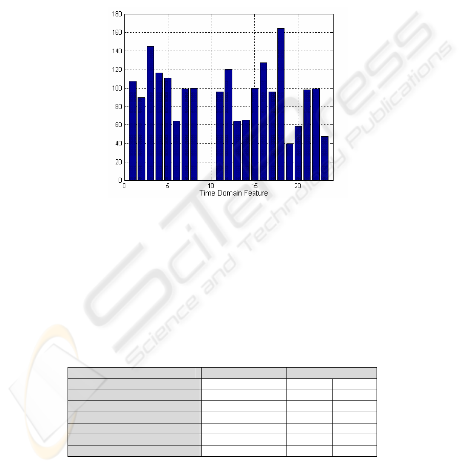
To estimate the best combinations of time domain features plus total spectral
energy, test errors of all 2²³ combinations were calculated. The distribution frequency
of the features in the 200 combinations with the best classification results was
calculated and plotted on a histogram (figure °3). Additionally, the five best
combinations are shown in table °3. The results point out a high variability of features
in these combinations, which makes a judgment of every single feature impossible.
Just the low frequency of features involved in the 200 feature combinations with
minimal test error (figure °3) leads to the worse classification ability of some features.
Fig. 3. Absolute frequency of 200 best feature numbers. From all 2²³ feature combinations 200
with the lowest test error were extracted to estimate the classifiability of each single feature. A
high frequency of a feature means good classifiability
The best five combinations of time domain feature extraction methods and the best
two from the spectral domain, namely MTM and Burg, were than used to examine the
optimal classification method. At all classification methods, we empirically estimated
the number of neurons to minimize the estimation error.
Table 4. Results of the comparison of classification methods (TDX = x-th combination of time
domain feature extraction methods). Results point out two classification methods to be suitable:
For spectral domain OLVQ, for time domain GCS. Results of GCS show a very high variance
and a much higher test error at all
feature extraction method class. method E
TEST
[%]
Burg OLVQ 2,2 ± 0,0
MTM OLVQ 8,0 ± 0,5
TD1 GCS 16,7 ± 4,5
TD2 GCS 29,8 ± 10,8
TD3 GCS 23,7 ± 6,6
TD4 GCS 23,8 ± 8,6
TD5 GCS 20,8 ± 6,3
47

Analysis of the results pointed out that two methods seem to be suitable. For
spectral domain it was OLVQ, for time domain GCS (table °4). For computing the
remaining combinations of the study, just the Burg Method for feature extraction and
OLVQ for classifying were used, because all other methods showed a considerably
higher test error.
3.2 Evaluation of the study
All trials were binary tested against each other, so the neural networks had to solve
two-class problems with an a priory test error of 50%. Our assumption was, that the
different trial modalities are, the better classification results (low test error) would be.
For instance, 00 vs. 11 and 00 vs. 12 should be good classifiable because every
modality differs, 11 vs. 12 should be the opposite, because the modalities here are
rather the same.
Table °5 gives an overview over the results. In opposition to our assumption, 00 vs.
10 showed the lowest test error. All other results accord with it, but the great
difference between combination 2 and 3 seems to be inexplicable, because the
modalities between both combinations differed only in length of the binaural
stimulation, plus all subjects reported equal feelings. However, the results of 11 vs. 12
confirm our assumption once more, leading to high test errors when modalities equal
Table 5. Results of study. For each classified trial the optimal number of neurons is given,
estimated empirically. The custom “eyes open vs. eyes closed” combination showed best
results, against our expectation that 00 vs. 11 or 00 vs. 12 would do this
classified trials # neurons E
TEST
[%]
00 vs. 10 95 4,2 ± 1,8
00 vs. 11 22 9,6 ± 2,0
00 vs. 12 60 16,2 ± 2,9
10 vs. 11 55 17,3 ± 2,7
10 vs. 12 97 20,2 ± 3,1
11 vs. 12 97 23,8 ± 2,8
4 Conclusion
Postural sway of nine healthy volunteers was measured in four trials with different
modalities of visual feedback and binaural stimulation. Raw data was segmented in
order to multiply data for the classification methods and beware stationarity of the
signal. 15 different feature extraction methods of time and spectral domain were
applied than to the segmented data. Parameters of these methods, including feature
combination in time and frequency band in spectral domain, were optimized by
minimizing the empirical error. The best combinations of time domain feature
extraction methods and the best from the spectral domain were than used to examine
the optimal classification method. It turned out, that Burg autoregressive method of
power spectral density estimation and Optimized Learning Vector Quantization was
the best method combination. The classification task “no impairment” versus “visual
48

impairment”, i.e. “eyes open” versus “eyes closed”, showed best discriminative
performance indicated by mean test errors of 4.2%.
In comparison to spectral domain, time domain features showed an unexpectable
low performance, for which we have no explanation. In our opinion technical
limitations play no role, in addition our system is technically improved, with a
exceptionally high sampling rate of 1000 sec
-1
and a 14 bit resolution in AD
converter. Also the task duration of 100 sec is higher in comparison to other authors,
the utilized classification algorithms are very adaptive and are much more sensitive
than every group oriented statistic. It is astonishing that spectral features perform so
much better than time domain features. Mean test errors of 4.2% are an extraordinary
performance in the domain of stochastic biosignals. The pilot study pointed out, that
the established biosignal analysis system gained a high sensitivity on small postural
influences. Future work should be oriented on investigation on more subjects and
more repetitive measurements over several weeks.
References
1. Chiari, L., Rocchi, L. and Cappello, A.: Stabilometric parameters are affected by
anthropometry and foot placement. Clinical Biomechanics (2002) 666-677
2. Clair, K.L. and Riach, C.: Postural stability measures: what to measure and for how long.
Clinical Biomechanics (1996) 176-178
3. Collins, J.J. and De Luca, C.J.: Upright, correlated random walks: A statistical-
biomechanics approach to the human postural control system. Chaos (1995) 57-63
4. Fransson, P.A. et al.: Adaption to vibratatory perturbations in postural control. IEEE
engineering in medicine and biology Magazine (2003) 53-57
5. Fritzke, B.: Vektorbasierte Neuronale Netze. Universität Erlangen - Nürnberg (1998)
6. Harris, C.S.: Effects of increasing intensity levels of intermitted and continuous 1000 Hz
tones on human equilibrium. Perceptual and Motor skills (1972) 395-405
7. Joachims, T.: Learning to classify text using support vector machines.
KluwerAc.Pub.(2002)
8. Kohonen, T.: Learning Vector Quantization. Neural Networks (1988) 303-306
9. Kohonen, T.: Self organizing maps. Berlin, Heidelberg, New York: Springer Verlag (2001)
10. Loughlin, P.J. and Redfern, M.S.: Spectral characteristics if visually induced postural sway
in healthy elderly and healthy young subjects. IEEE Trans.Neur.Sys. (2001) 24-30
11. Loughlin, P. and Redfern, M.: Analysis and modelling of human postural control. IEEE
Engineering in Medicine and Biology Magazine (2003) 18
12. Nakagawa, H. et al.: The contribution of proprioception to posture control in normal
subjects. Acta Otolaryngol (1993) 112-116
13. Oie, K.S. et al. Multisensory fusion: simultaneous re-weighting of vision and touch for the
control of human posture. Cognitive Brain Research (2002) 164-176
14. Oostervelt, W.J., Polman, A.R. and Schoonheyt, J.: Vestibular implications of noise-inducd
hearing loss. British Journal of Audiology (1982) 227-232
15. Percival, D.B. et al. : Spectral analysis for physical applications. Cambridge University
Press (1993)
16. Raper, S.A. and Soames, R.W.: The influence of moving auditory fields on postural sway
behaviour in man. European Journal of Applied Physiology (1992) 241-245.
17. Sakellari, V. and Soames, R.W.: Auditory and visual interactions in postural stabilization.
Ergonomics (1996) 634-648
18. Vapnik, V.: Statistical Learning Theory. Chichester, GB: Wiley (1998)
49
