
Optimizing ICA Using Prior Information
Giancarlo Valente
1,2
, Giuseppe Filosa
1
, Federico De Martino
2
, Elia Formisano
2
,
Marco Balsi
1
1. Department of Electronic Engineering, University of Rome “La Sapienza”, Italy.
2. Department of Cognitive Neuroscience, University of Maastricht, The Netherlands.
Abstract. In this work we introduce a novel algorithm for Independent
Component Analysis (ICA) that takes available prior information on the sources
into account. This prior information is included in the form of a “weak”
constraint and is exploited simultaneously with independence in order to
separate the sources. Optimization is performed by means of Simulated
Annealing. We show how it outperforms classical ICA algorithms in the case of
low SNR. Moreover, additional prior information on the sources enforces the
ordering of the components according to their significance.
1 Introduction
Independent component analysis (ICA) is a technique that aims to separate
statistically independent signals from the observation of an (unknown) linear mixture
of these signals [1]. No a priori assumptions are usually made on the underlying
sources or on the mixing, except for the statistical independence of the original
signals.
Since its introduction ICA has been used successfully in several research fields.
Recently ICA has received great attention in various fields of functional
neuroimaging, including functional magnetic resonance imaging (fMRI) and electro-
and magneto-encephalography (EEG,MEG) [2],[3]. In all cases, observed data x are
modeled as a linear mixture of n statistically independent signals s: x=As where A is
the mixing matrix.
ICA algorithms attempt to recover the original sources by finding an estimate of
the unmixing matrix W such that the signals y=Wx are as much independent as
possible. However, due to the double indeterminacy in the mixing matrix and in the
original signals, it is not possible to define the variance of the sources univocally. For
the same reason, every permutation of the sources is still a solution, therefore no
intrinsic ordering of the sources is defined (unlike in principal component analysis,
where signals are extracted according to the amount of variance they explain). Several
algorithms have been proposed, using high order statistic (HOS) or second order
statistics (SOS), based on information theory criteria or on decorrelation principles.
For a review, see [4],[5].
Valente G., Filosa G., De Martino F., Formisano E. and Balsi M. (2005).
Optimizing ICA Using Prior Information.
In Proceedings of the 1st International Workshop on Biosignal Processing and Classification, pages 27-34
DOI: 10.5220/0001195800270034
Copyright
c
SciTePress

While performances of conventional hypothesis-driven techniques highly depend
on the accuracy of a predefined model/template, the generality and the nature of the
assumptions underlying ICA make it a powerful and flexible tool. Some kind of
general knowledge of the sources, however, is often available [6]. In fMRI, for
instance, interesting sources of brain activity are expected to show regularities in
space and time. Similar considerations also apply to a broader range of ‘mixtures’ of
natural signals, in which interesting sources have some form of regularity. Such
information is completely ignored in classical ICA, as the structure of data does not
influence the cumulative statistics employed in the algorithm.
Prior information on a source together with gradient optimization has been used to
influence the order of extraction of the components ([7], [8], [9]) and to recover their
real variance (constrained ICA, [8]). In [9] the knowledge of reference functions of
different paradigms is incorporated into the extraction algorithm in order to perform a
semi-blind ICA. However, these approaches employ specific and rather strong
information on the sources and thus are affected by the same drawbacks as in the case
of hypothesis-driven methods,
In this paper, we propose an approach that allows including in ICA prior
knowledge of the spatial/temporal structure of the sources in a systematic and general
fashion. Such prior information can be quite general, so as to apply broadly to
potentially interesting signals, without requiring detailed knowledge of source
properties. The proposed solution also enforces the ordering of the extracted
components according to their significance. This is an advantage when only few of a
large number of components are actually interesting for the interpretation of the data.
2 ICA with Prior Information
The solution of an ICA problem can be obtained in two steps: defining a suitable
contrast function that measures independence, and optimizing it.
To avoid the direct computation of probability density functions, information-
theory-based contrast function are used. In particular robust estimates of mutual
information and negative entropy are employed to determine the degree of
independence between the estimated signals. Using the central limit theorem, it has
been shown that a linear transformation of the data that maximizes non-Gaussianity,
leads to independence as well [4].
FastICA recovers the sources by maximizing an estimate of negative entropy,
which is a measure of non-Gaussianity, by means of a fixed-point iteration algorithm.
In particular, negative entropy is approximated as follows:
()
(
)
(
)
{
}
[
]
2
ν
GyGyJ
G
−Ε=
(1)
where ν is a Gaussian distributed signal with the same mean and variance as y.
Maximization can be performed considering all the output signals together
(symmetric approach), or extracting one source at a time using a deflation approach.
Our approach is based on the maximization of a novel contrast function F:
28

HJF
λ
+
=
(2)
where J is again an estimate of negative entropy, and H accounts for the prior
information we have on sources. The parameter λ is used to weigh the two parts of the
contrast function. If λ is set to zero, maximization of F leads to pure independence.
As is usual with regularization problems, λ must be chosen appropriately to ensure
that both parts of the function are actually active. This problem is also related to the
fact that the magnitude of J and H must be appropriately limited and normalized. We
consider two basic approaches for the choice of H, according to the type of constraint
that should be enforced. H can be a nonlinear saturating function or a monotonic one.
A saturating H is only active in a limited domain, so that we obtain a constrained
optimization algorithm, in which independence is optimized freely within a bounded
class of functions. The second case, instead, requires joint optimization of the two
conditions, and is more sensitive to the choice of λ.
In order to keep the method as general as possible, it is preferable not to impose H
to be differentiable. Therefore we choose to maximize the contrast function using
Simulated Annealing (SA), a well known optimization procedure that has proved to
be a really powerful tool for optimization problems [11],[12].
The main advantage of SA is that it does not require use of derivatives to reach the
global optimum, even if it usually requires more time if compared with gradient
optimizations. Optimization is performed considering one component at a time, and
decorrelating the subsequent components at each iteration.
3 Methods
To test our algorithm we used a simulated fMRI dataset, consisting of three different
activation maps with related time courses (Fig. 1). The three maps were sparse, highly
localized and not overlapping; therefore all the assumptions of ICA model were met.
The three sources were mixed up, and FastICA managed to extract them exactly if
no noise was superimposed. As shown in [13], performance of classical ICA
algorithms tends to deteriorate as the SNR of the sources decreases.
In order to improve separation performances in case of superimposed noise we
performed new extractions including an additional term to account for prior
information on the spatial and temporal structure of the sources. We considered three
different contrast functions H that considered the spatial one-lag autocorrelation,
temporal one-lag autocorrelation and a linear combination of them. Such information
is meant to describe very loosely the regularity of natural signals. Let the two
dimensional index p refer to the image, then the spatial one-lag autocorrelation can be
expressed as:
()
]))(([#)()()(
2
ypNkypyyH
ppNk
sp
⋅⋅=
∑∑
∈
(3)
29

where N(p) is the 1-neighborhood of point p, and #N(p) is the cardinality of the
neighborhood.
The temporal one-lag autocorrelation of vector w can be calculated as:
()
(
)
2
1)( wtwtwwH
t
t
∑
+⋅=
(4)
In the first case we considered a purely spatial constraint, in the second a purely
temporal one, while in the third we considered a spatio-temporal constraint.
Sources that have spatial and temporal structure are expected to have higher values
of the contrast function so that their extraction is enhanced.
To test the algorithm we considered two different frameworks: in the first we
added Gaussian white noise to the mixed sources, and studied performances
according to the level of noise introduced, while in the second we superimposed the
artificial activations to a resting state experiment, modifying the amplitude of the time
courses of the injected activations.
In both case we evaluated the correlation between the original sources and the
recovered ones as a measure of the effectiveness of the extraction.
3.1 Test on Artificial Activations with Gaussian White Noise
We considered different levels of noise, and for each level the correlation between the
estimated source and the corresponding original one was computed. As expected,
FastICA performance deteriorates considerably and rather abruptly as the SNR of the
independent sources decreases. Instead, considering additional general prior
information such as high spatial and/or temporal autocorrelation makes the overall
extraction performances better.
In this case the additional contrast function H was weighted two orders of
magnitude more than pure independence, but considered until a threshold, so that we
looked for the maximization of negentropy within a subset of the original domain
such that H was above threshold.
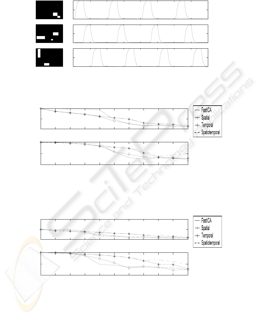
In Figs. 2-4 the correlation of each spatial source with the corresponding separated
component vs. power of noise is depicted in the top panel, while in the bottom
correlation of corresponding time-courses is shown.
Correlation was calculated on thresholded maps, and each of the four algorithms
was executed 6 times, to give more significance to results.
The continuous line corresponds to FastICA extraction, the continuous-plus one to
the one-lag spatial autocorrelation additional cost function, the continuous-diamond to
one-lag temporal autocorrelation, while the dashdot line indicates the linear
combination of both cost functions. It is evident that spatial autocorrelation is more
effective in this setting.
As shown in Figs. 2-4, for high levels of noise the incorporation of prior
information helps recovering the sources more effectively, while classical
independence search fails to identify the sources. Performance decay of the
constrained algorithm is more regular with noise appearing almost linear.
30
0 10 20 30 40 50 60 70 80
0 10 20 30 40 50 60 70 80
0
10
20
30
40
50
60
70
80
Fig. 1. Simulated spatial independent sources with corresponding time courses (active voxels in
white).
0 0.2 0.4 0.6 0.8 1 1.2 1.4 1.6 1.8 2
0
0.5
1
First Source
Correlation
0 0.2 0.4 0.6 0.8 1 1.2 1.4 1.6 1.8 2
0
0.5
1
Variance of noise
Correlation
Fig. 2. Values of correlation between the first original source and the corresponding estimated
one.
0 0.2 0.4 0.6 0.8 1 1.2 1.4 1.6 1.8 2
0
1
2
Second Source
Correlation
0 0.2 0.4 0.6 0.8 1 1.2 1.4 1.6 1.8 2
0
0.5
1
Variance of noise
Correlation
Fig. 3. Values of correlation between the second original source and the corresponding
estimated one.
31

0 0.2 0.4 0.6 0.8 1 1.2 1.4 1.6 1.8 2
0
0.5
1
Third Source
Correlation
0 0.2 0.4 0.6 0.8 1 1.2 1.4 1.6 1.8 2
0
0.5
1
Variance of noise
Correlation
Fig. 4. Values of correlation between the third original source and the corresponding estimated
one.
3.2 Test on Artificial Activations Superimposed to Resting State fMRI
Experiment
We considered in this case a fMRI resting state experiment performed by a healthy
volunteer. The whole brain was acquired on a 3T Siemens Allegra (Repetition Time
1.5s, Interslice time 46 ms, 32 slices, matrix 64×64, slice thickness 3mm, 210
volumes). We skipped the first two volumes due to T2* saturation effects, and
performed a linear de-trending and high pass filtering with BrainvoyagerQX.
We therefore added the three simulated activities a single slice of the collected
dataset. In this case we modified the amplitude of the time courses of the simulated
activity at different Contrast to Noise Ratios (CNR), where CNR is the ratio of signal
enhancement and the standard deviation of the fMRI time series in those voxels that
are active. It is known in literature [13] that as the CNR decreases below 1, ICA
performances in fMRI signal extraction deteriorate significantly.
In this case we weighted the additional contrast function H an order of magnitude
less than negentropy (independence), because of the presence of other spatially and
temporally autocorrelated sources already present in the resting state dataset and
related to various causes (like movement artifacts, vessels), and that have higher
power than the simulated activations. As in the previous case, we considered the
correlation between sources and recovered signals as a benchmark for the separation.
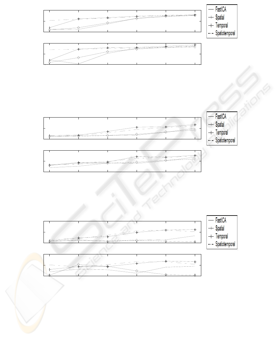
In Figs. 5-7 correlations between the original sources and the recovered ones are
depicted for CNR ranging from 0.5 to 1. It has to be noted that also in this case the
new contrast function term helps recovering the sources even in the case when
FastICA fails to identify them.
Poor performances of temporal autocorrelation additive contrast function may be
due to the small number of time samples considered (100 points), while spatial
autocorrelation was computed over a whole slice (consisting of 4096 points).
32
0.5 0.6 0.7 0.8 0.9 1
0
0.5
1
First source
correlation
0.5 0.6 0.7 0.8 0.9 1
0
0.5
1
contrast to no i se rati o
correlation
Fig. 5. Values of correlation between the first original source and the corresponding estimated
one (top panel) and between time courses (bottom panel).
0.5 0.6 0.7 0.8 0.9 1
0
0.5
1
Seco nd so urce
correlation
0.5 0.6 0.7 0.8 0.9 1
0
0.5
1
contrast to no i se rati o
correlation
Fig. 6. Values of correlation between the second original source and the corresponding
estimated one (top panel) and between time courses (bottom panel)
0.5 0.6 0.7 0.8 0.9 1
0
0.5
1
Third source
correlation
0.5 0.6 0.7 0.8 0.9 1
0
0.5
1
contrast to noise ratio
correlation
Fig. 7. Values of correlation between the second original source and the corresponding
estimated one (top panel) and between time courses (bottom panel)
33

4 Conclusions
In this work we propose an approach to incorporate available prior information into
independent component analysis. This approach has the advantage of being very
general and flexible, as prior information is included in the form of an additional cost
function of any kind. The proposed method can be used for a wide area of problems
where there is some kind of prior knowledge on the sources, either considering
information as an additional contrast function, or considering it as a constraint. In
addition, we have shown that it is possible to enhance source extraction by using
general cost functions, like spatial one-lag autocorrelation and/or temporal one-lag
autocorrelation, without having detailed information on some of the sources, and
making the extraction more robust with respect to additive noise.
References
1. P. Comon: Independent component analysis—A new concept?, Signal Processing, (1994)
36(3), 287–314.
2. T.P. Jung, S. Makeig, MJ McKeown, A.J. Bell, T.W. Lee, T.J. Sejnowski: Imaging brain
dynamics using independent component analysis, Proceedings of the IEEE, (2001), 89(7)
1107-22.
3. M.J. McKeown, S. Makeig, G.G. Brown, T.P. Jung,S.S. Kindermann, A.J. Bell, T.J.
Sejnowski: Analysis of fMRI data by blind separation into spatial independent component
analysis. Human Brain Mapping (1998), 6, 160-188.
4. A. Hyvärinen, J. Karhunen, E. Oja: Independent Component Analysis, Wiley, 2001
5. A. Cichocki, S.I. Amari: Adaptive Blind Signal and Image Processing, Wiley, 2002
6. M.J. McKeown, T.J. Sejnowski: Independent component analysis of fMRI data: examining
the assumptions. Human Brain Mapping (1998), 6, 368-372
7. C. Papathanassiou, M. Petrou: Incorporating prior knowledge in ICA, Digital Signal
Processing 2002. IEEE 14th Int. Conf. On, (2002) 2, 761.64.
8. W. Lu, J. Rajapakse: Eliminating indeterminacy in ICA, Neurocomputing (2003), 50, 271-
290.
9. V.D. Calhoun, T. Adali, M.C. Stevens, K.A. Kiehl, J.J. Pekar: Semi-blind ICA of fMRI: a
method for utilizing hypothesis-derived time courses in spatial ICA analysis, Neuroimage,
(2005), 25(2), 527-538.
10. A. Hyvärinen: Fast and Robust Fixed-Point Algorithms for Independent Component
Analysis, IEEE Trans. on Neural Networks, (1999), 10(3), 626-634.
11. S. Kirkpatrick, C. D. Gelatt, Jr., M.P. Vecchi: Optimization by simulated annealing,
Science, (1983), n. 4598,.
12. Handbook on algorithms and theory of computation, M.J. Atallah editor, CRC Press,
(1998).
13. F. Esposito, E. Formisano, E. Seifritz, R. Goebel, R. Morrone, G. Tedeschi, F. Di Salle:
Spatial independent component analysis of functional MRI time-series: To what extent do
results depend on the algorithm used?, Human Brain Mapping, (2002) 16(3), 146-157.
34
