
A Randomized Gathering Algorithm for Multiple
Robots with Limited Sensing Capabilities
⋆
Noam Gordon, Israel A. Wagner and Alfred M. Bruckstein
Center for Intelligent Systems, CS Department
Technion — Israel Institute of Technology
Haifa 32000, Israel
Abstract. Consider a swarm of weak, anonymousandhomogeneousrobotslack-
ing memory, orientation, and communication capabilities, and having myopic
sensors that tell them the directions to nearby robots, but not the distance from
them. We present a simple randomized algorithm which, when performed by all
members of the swarm, gathers them in a small region. We explore the interesting
global phenomena that occur during the process, evident from our analysis and
simulations.
1 Introduction
In this paper, we present a very simple algorithm that makes a swarm of very simple
robots perform a seemingly simple task — getting together in a small region. From a
practical standpoint, it can be useful for collecting multiple ant-robots after they have
performed a task in the field; for enabling them to start a mission, after being initially
dispersed (e.g., parachuted); or for aggregating many nano-robots in a self-assembly
task. From a theoretical standpoint, it is the most basic instance of the formation prob-
lem, i.e., the problem of arranging multiple robots in a certain spatial configuration.
While advanced intelligent robots are certainly capable of gathering, the problem is
most challenging when the robots are ant-like or less — having very limited abilities,
e.g., myopic, disoriented and lacking explicit communication capabilities.
Several theoretical works on this subject exist. Current approaches include agree-
ment on a meeting point with some unique geometrical property [1–4]; using a common
compass [5]; cyclic pursuit [6–8]; and others [9–11]. Sugihara et al. suggested a simple
way to fill a convex shape, which is also useful for gathering [12].
These methods rely on strong assumptions about the robots (or agents as we shall
call them henceforth): Some rely on labeling (e.g., pursuit), some on common orienta-
tion, and many on infinite-range visibility. Nearly all works rely on the agents’ ability
to measure their mutual distances.
In this work, we suggest a simple gathering algorithm, which relies on very few
capabilities: Our agents are anonymous, homogenous, memoryless, asynchronous, my-
opic and are incapable of measuring mutual distances. We are not aware of previous
works using this limited model. The inspiration and motivation for this work came from
⋆
This research was partly supported by the Ministry of Science Infrastructural Grant No. 3-942.
Gordon N., A. Wagner I. and M. Bruckstein A. (2005).
A Randomized Gathering Algorithm for Multiple Robots with Limited Sensing Capabilities.
In Proceedings of the 1st International Workshop on Multi-Agent Robotic Systems, pages 56-63
DOI: 10.5220/0001194500560063
Copyright
c
SciTePress

experiments with real robots in our lab [13], made from LEGO parts and very crude
sensors, which are range-limited and do not provide usable distance measurements.
In [14], we presented a simple deterministic gathering algorithm, which is similar
in idea to the aforementioned polygon-filling algorithm of Sugihara et al., yet it has
the additional property of maintaining mutual visibility between the robots, in order to
cope with their shortsightedness. In this work, we present a randomized variant of the
algorithm. Due to space restrictions, we omitted the proofs and abridged the discussion.
More details can be found in [14] and in an upcoming extended paper.
2 Model and Algorithm
We begin with a definition of the world model. Then, we discuss the conditions which
guarantee that visibility is maintained between our myopic agents, and present the pro-
posed algorithm.
2.1 Model
The world consists of the infinite plane IR
2
and n point agents living in it. We adapt
Suzuki and Yamashita’s convenient way of modeling a system of asynchronous agents
[4]: Time is a discrete series of time steps t = 0, 1, . . .. In each time step, each agent
may be either awake or asleep, having no control over the random scheduling of its
waking times. A waking agent senses its environment, and is able to move instantly to
any point within a distance σ (the maximum step length). The agent is able to see other
agents within distance V (the visibility radius or range). However, it cannot measure its
distance from them. It only knows the directions in which the nearby agents are found,
i.e., the input is a cyclic list of angles θ
1
, . . . θ
m
(relative to some arbitrary direction,
e.g., the agent’s heading). There are no collisions. Several agents may occupy the same
point.
1
All agents are memoryless, anonymous (indistinguishable in their appearance)
and homogenous (they lack any individuality or identity, and perform the same algo-
rithm).
Regarding the agents’ activity schedule, we only assume that the agents are strongly
asynchronous: For any subset G of the agents and in each time step, the probability that
G will be the set of waking agents is bounded from below by some constant ε > 0.
Define the mutual visibility graph as an undirected graph with n vertices, represent-
ing the agents, and an edge between each pair of agents, if and only if they can see each
other, i.e., the distance between them is at most V .
2.2 Maintaining Visibility
We now present a sufficient condition, on any algorithm, for maintaining mutual visi-
bility between agents. In what follows, denote a disc of radius r and center a (where a
may signify the location of an agent a) by B
r
(a). Also, denote
µ ≡ min (V/2, σ) .
1
In this case, they have undefined relative directions and simply ignore each other.
Let agent a see m agents b
1
, . . . b
m
, and define the allowable region AR(a) of a:
AR(a) ≡ B
µ
(a) ∩
m
\
i=1
B
V/2
a +
V
2
·
b
i
− a
kb
i
− ak
. (1)
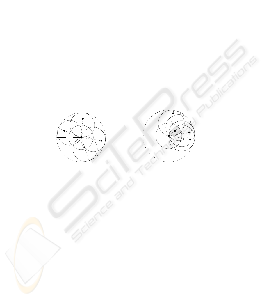
It is easily seen (cf. Fig. 1) that AR(a) is not empty if and only if all visible agents are
contained within a sector or “wedge” of less than half the disc B
V
(a), i.e., its angle is
less than π. In this case, AR(a) is simply the intersection of B
µ
(a) and the two discs
corresponding to the agents on the wedge’s bounds (e.g., b
1
and b
4
in Fig. 1(b)):
AR(a) = B
µ
(a) ∩B
V/2
a +
V
2
·
b
1
− a
kb
1
− ak
∩B
V/2
a +
V
2
·
b
m
− a
kb
m
− ak
. (2)
Also, if m = 0, then AR(a) = B
µ
(a). The following lemma holds.
Lemma 1. If each agent confines its movements to the allowable region defined above,
then existing visibility will be maintained.
V
b
1
b
2
b
4
b
3
a
(a)
V
b
3
b
4
a
b
1
b
2
(b)
Fig.1. Maintaining visibility. (a) a is surrounded and cannot move (AR(a) = ∅). (b) a can move
only within the shaded area.
2.3 The Algorithm
The proposed algorithm is as follows:
Move to a uniformly-distributed random point in the allowable region (unless
it is empty, in which case do not move).
Interestingly, the algorithm doesn’t seem to “care” for anything but maintaining
visibility, yet its rationale is similar to that of the deterministic algorithm from [14]
(where the agent moves as far as allowed along the bisector of the wedge): The agents
inside the area occupied by the swarm do not move, while the agents at the outskirts
move inside, making the swarm shrink, until all agents are gathered densely in a small
cluster.
3 Results and Analysis
Despite its extreme simplicity, the algorithm effectively manages to gather all agents in
a small cluster. Moreover, we observed in our simulations some very interesting global
phenomena, which we discuss in this section.
−20 0 20 40 60 80
−50
0
50
t = 0
−20 0 20 40 60 80
−50
0
50
t = 40
−20 0 20 40 60 80
−50
0
50
t = 150
20 25 30 35 40
−5
0
5
10
15
20
t = 800
31 32 33 34 35
7
8
9
10
11
12
t = 1300
32.2 32.4 32.6 32.8 33 33.2
8.6
8.8
9
9.2
9.4
9.6
t = 1500
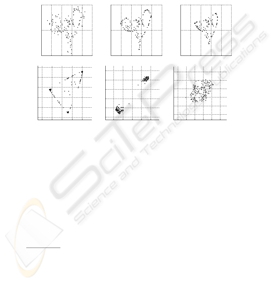
Fig.2. A typical run. Here n = 150, σ = 1, V = 10, and each agent wakes up in each time step
with probability p = 0.6. Note that the scale changes between frames.
3.1 Global Behavior
The qualitative behavior of the algorithm is clearly divided into two phases (similarly
to the deterministic variant). First, in the contraction phase, the area occupied by the
agents contracts into a small dense cluster
2
. In a large swarm, the contraction process
exhibits an interesting behavior, where the occupied area shrinks non-uniformly, as-
suming an approximate polygonal shape with a few corners and roughly straight edges
between them (cf. Fig. 2). The corners are actually dense clusters of several agents. The
edges are “belts”, containing the agents that were swept by the contracting boundary.
The density of agents along the edges is much lower than in the corners. More gener-
ally, there is a correlation between high curvature (of the boundary) and high density
2
We use the term “area occupied by the agents” freely, as a subjective observation of the agents’
distribution or the shape of the swarm. It can be defined formally as the area enclosed by
laying line segments between all pairs of mutually visible agents. When all agents are mutually
visible, this area equals the convex hull of the agents’ locations. An alpha-shape may also be
considered, however its parameter α has no clear meaning in our problem.
of agents. We believe that there is a positive-feedback relationship between density and
curvature, which results in the large-scale polygonal shape, having sharp dense corners
and linear edges of lower density.
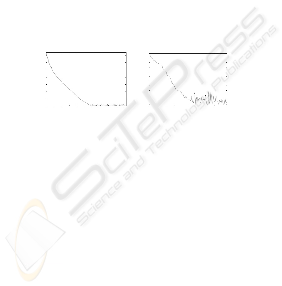
The occupied area contracts until it becomes a small dense cluster with a mean
diameter
3
of about µ. At this stage, the wandering phase begins. The dense cluster
stops contracting, and begins wandering in the plane, instead. The reason to this change
is clear: The agents’ step sizes are not affected by the scale of the occupied area. As
long as the area is large in comparison to µ, the agents on its boundary generally move
inside it, making it contract. However, once the area becomes smaller, the agents’ steps
become relatively larger, so they leap over it, instead. As a result of these leaps, the
cluster drifts along the plane indefinitely. Note that since there is full visibility between
the agents at this stage, only the agents at the vertices of the convex hull are able to
move.
100 200 300 400 500 600 700 800 900 1000
5
10
15
20
25
30
35
time
diameter
(a)
500 520 540 560 580 600 620
0.6
0.8
1
1.2
1.4
1.6
1.8
2
2.2
2.4
2.6
time
diameter
(b)
Fig.3. The diameter in a typical run of the algorithm. Here n = 60, σ = 1, V = 5, and p = 0.6.
(a) The phase transition is very clear. (b) Zooming in on the transition moment. Note that the
mean diameter is about 0.8µ after the transition.
When n ≤ 2, the two algorithm variants act differently. In the deterministic algo-
rithm, a single agent will not move, and a pair will always remain on one line. In the
randomized variant, the agents will roam the plane in either case.
3.2 Guaranteed Convergence
The following theorem holds (We omitted the proof for space considerations).
Theorem 2. Given an initial configuration with a connected visibility graph, the agents
will gather and forever remain in a cluster whose diameter is bounded by V , in finite
expected time.
The proof idea is as follows: We show that, in every time step, there exists an agent
(specifically, one located at a vertex of the convex hull), which has a strictly positive
4
3
The term mean diameter here refers to the average diameter over time (in a given run), not
probability space.
4
i.e., positive and bounded away from zero by some constant.

chance of moving inside the convex hull and closer to the center of mass (average of the
agents’ positions) by a strictly positive amount, if it is the only agent which wakes up.
By our strong asynchronicity assumption, the chance that this will happen is also strictly
positive (bounded by ε). This, in turn, will make the variance (sum of squared distances
from the center of mass) decrease by a strictly positive amount. Thus, with time, the
variance will decrease arbitrarily with probability 1. As the variance gets smaller, the
diameter must too, so at some point, the diameter will be V or less, which implies that
the visibility graph is a clique. By Lemma 1, it will remain a clique, and therefore the
diameter will remain bounded by V .
3.3 Evaluation of the Mean Cluster Diameter
Theorem 2 guarantees gathering to diameter V . However, the simulations clearly show
further contraction to a mean diameter of about 0.8µ during the wandering phase
5
, fairly
indifferently to the choice of n. With the deterministic algorithm, the mean diameter
typically settles at about 1.04µ.
When the agents are scattered (i.e., the diameter is much larger than µ) the diameter
is much more likely to decrease, and when the agents are gathered in a small cluster, it is
likelier to increase (e.g., consider a limit case of an infinitesimally small cluster). Thus,
we infer that there exists a probabilistically stable equilibrium point for the diameter.
This point is the expected mean diameter.
An exact calculation of the expected mean diameter seems to be difficult, yet the
following rough estimate for large n provides a surprisingly good prediction of the
measured results. Given a dense cluster P with diameter D(P ) ≪ V , we first approxi-
mate its convex hull shape as a disc of diameter D(P ). The corner agents reside on its
boundary, with their wedge bisectors pointing to its center. We assume that σ ≪ V and
n is large, so that the allowable region of each corner agent is approximately a narrow
sector (i.e., a “pizza slice”) of a disc of radius µ. Now, we approximate the expected
mean diameter as that for which, for each corner agent, the probability of moving into
the convex hull equals the probability of leaping over it. Geometrically, it means that
the intersection of the narrow sector and the disc should contain half of the sector’s area.
This holds when the disc’s diameter is about µ/
√
2, which is quite close to the observed
typical mean diameter of 0.8µ.
In the deterministic variant of the algorithm, assuming that σ is small enough, the
agent simply moves a step of size µ on the bisector (i.e., along the disc’s diameter in our
approximation). Thus, the expected mean diameter is simply µ. Again, it agrees well
with the measured typical mean diameter of 1.04µ.
3.4 Composite Random Walking
The random wandering of the cluster is composed of the movements of the individual
agents in it (hence we term it a composite random walk). An interesting question is
5
Although we determined the moment of phase transition subjectively, it is evident from Fig. 3
that this moment is very clear. We calculated the average diameter from about 20 time steps
ahead of that moment until the end of the simulation (several hundred steps later).

whether this random walk is recurrent or not. Based on our observations, we conjecture
that it is indeed. If so, then it has a very important implication: Theorem 2 guarantees
that a configuration with a connected visibility graph will contract. Thus, in the general
case, each connected component will contract into an independent cluster. Now, if the
cluster’s random walks are recurrent, then they will all meet eventually and merge into
one cluster.
In order to be recurrent, a two-dimensional random walk needs to be unbiased.
Obviously, when observing a single time step, the random movement is not distributed
uniformly in all directions, as it depends on the exact shape of the convex hull. However,
when integrating over many time steps, one may show that the cluster’s displacement is
distributed uniformly in all directions.
A single isolated agent performs a uniform random walk by definition. For two
agents, observe that the probability distribution of the center of mass’s displacement
is always symmetric along the line passing through the two agents, and has a constant
shape up to its orientation in the plane. Thus, the change of orientation has a con-
stant and unbiased distribution (i.e., same for clockwise and counterclockwise changes).
Therefore, over time, the orientation will be distributed uniformly, and, accordingly, the
center of mass’s displacement distribution will approach uniformity as well.
For n > 2, unfortunately, we don’t have an easy proof. Even with only three agents,
the state-space becomes complex and hard to analyze. Again, we conjecture that the
composite random walk of three or more agents is indeed recurrent. This seems to be
the case from observing long runs of the simulations.
4 Conclusions
The main contribution of our work is that we consider the gathering problem with such
severe limits on the agents’ sensors (being both myopic and unable to measure dis-
tances), in addition to being anonymous and memoryless. The proposed algorithm is an
example of how deceptively simple individual behaviors can yield complex emergent
global behaviors of the swarm — two distinct phases of contraction and wandering,
where the swarm first assumes an approximate polygonal shape and then collapses into
a dense cluster wandering in the plane.
If our conjecture regarding the recurrence of the composite random walk proves to
be true, then the algorithm is a very powerful one, gathering all agents together into a
dense cluster, regardless of their initial distribution. We find it intriguing that it does
that even though it is seemingly unconnected to the gathering problem, as the agents
just move randomly while trying to maintain their visibility. One may view this as an
argument that gathering is the only global task that such a swarm of weak robots can
do, i.e., it is a sort of an “upper bound” on the swarm behavior capabilities.
Further work should provide tighter estimates of the convergence rate, and analyze
the effect of noise and error, both in sensing and movement, on the resulting global
behavior.

References
1. Cieliebak, M., Flocchini, P., Prencipe, G., Santoro, N.: Solving the robots gathering problem.
In: Proc. of ICALP 2003. (2003)
2. Gordon, N., Wagner, I.A., Bruckstein, A.M.: Discrete bee dance algorithms for pattern for-
mation on a grid. In: Proc. of IEEE Intl. Conf. on Intelligent Agent Technology (IAT03).
(2003) 545–549
3. Schlude, K.: From robotics to facility location: Contraction functions, weber point, convex
core. Technical Report 403, CS, ETHZ (2003)
4. Suzuki, I., Yamashita, M.: Distributed anonymous mobile robots: Formation of geometric
patterns. SIAM Journal on Computing 28 (1999) 1347–1363
5. Flocchini, P., Prencipe, G., Santoro, N., Widmayer, P.: Gathering of autonomous mobile
robots with limited visibility. In: Proc. of STACS 2001. (2001)
6. Bruckstein, A.M., Cohen, N., Efrat, A.: Ants, crickets and frogs in cyclic pursuit. Technical
Report CIS-9105, Technion – IIT (1991)
7. Bruckstein, A.M., Mallows, C.L., Wagner, I.A.: Probabilistic pursuits on the grid. American
Mathematical Monthly 104 (1997) 323–343
8. Marshall, J.A., Broucke, M.E., Francis, B.A.: A pursuit strategy for wheeled-vehicle forma-
tions. In: Proc. of CDC03. (2003) 2555–2560
9. Ando, H., Oasa, Y., Suzuki, I., Yamashita, M.: A distributed memoryless point convergence
algorithm for mobile robots with limited visibility. IEEE Trans. on Robotics and Automation
15 (1999) 818–828
10. Lin, Z., Broucke, M.E., Francis, B.A.: Local control strategies for groups of mobile au-
tonomous agents. IEEE Trans. on Automatic Control 49 (2004) 622–629
11. Melhuish, C.R., Holland, O., Hoddell, S.: Convoying: using chorusing to form travelling
groups of minimal agents. Robotics and Autonomous Systems 28 (1999) 207–216
12. Sugihara, K., Suzuki, I.: Distributed algorithms for formation of geometric patterns with
many mobile robots. Journal of Robotic Systems 13 (1996) 127–139
13. The Center of Intelligent Systems, Technion IIT web site:
http://www.cs.technion.ac.il/Labs/Isl/index.html.
14. Gordon, N., Wagner, I.A., Bruckstein, A.M.: Gathering multiple robotic a(ge)nts with limited
sensing capabilities. Lecture Notes in Computer Science 3172 (2004) 142–153
