Cooperative Control Of A Robot Swarm With Network

Communication Delay

Yechiel Crispin

Department of Aerospace Engineering,

Embry-Riddle University, Daytona Beach, FL 32114, USA

Abstract. A new method for the cooperative control of a system of multiple

mobile robots with time delay in the network communication is presented. The

network of mobile robots is modeled as a swarm of particles performing a di-

rected random walk where the motion of the swarm is controlled by a central unit

such as a robot leader. The collective motion of the robots is modeled by a sys-

tem of stochastic delay-difference equations where the best solution found by the

swarm is used as the network cooperative control signal. The method is applied

to the solution of two problems. In the ﬁrst problem, a group of autonomous un-

derwater vehicles (AUVs) searches for the maximum depth in a two-dimensional

domain. In the second problem, the group of AUVs searches for the minimum

temperature in a three-dimensional domain. It is found that the search proceeds

along Levy ﬂights followed by sticking short random walks in the vicinity of the

extremum points and that the cooperative control method is robust to time delays

in network communication.

1 Introduction

In the past, robots have been used in many practical applications such as industrial ro-

bots in manufacturing, spacecraft and rover robots for space exploration and unmanned

air vehicles (UAVs) for reconnaissance, surveillance and tactical military missions.

Other possible applications include underwater missions by autonomous underwater

vehicles (AUVs) such as formation control and rendezvous, search and rescue missions

and exploration and mapping of unknown environments. At the beginning, single ro-

bots were employed in the performance of any given task. It has been recognized for

some time, however, that the use of collaborating multiple mobile robots can have sig-

niﬁcant advantages in achieving complex tasks and missions which otherwise might

not be achievable with single robots. Consequently, in recent years, researchers started

treating remarkable problems related to the cooperative control of networked collabo-

rating mobile robots with distributed resources such as sensors, computing power and

communications [1], [2] and [3].

The present paper represents a step in that direction. Consider a speciﬁc implemen-

tation of a group of mobile robots in the form of a group of auto-nomous underwater

vehicles, assigned with the collective task of exploring a limited domain of a body

of water such as a lake, sea or a limited part of the ocean. Let’s consider a speciﬁc

task where the robots have to collectively ﬁnd the extremum of an otherwise unknown

Crispin Y. (2005).

Cooperative Control Of A Robot Swarm With Network Communication Delay.

In Proceedings of the 1st International Workshop on Multi-Agent Robotic Systems, pages 3-14

DOI: 10.5220/0001193400030014

 SciTePress

function using a given experimental method where they can measure a property of the

environment such as water depth or temperature at any required point, see for exam-

ple [4] and [5]. The simplest such test problem is for the group of robots to collectively

search the maximum depth in a limited area; for example a group of 10 robots searching

an area of 1 km by 1 km and measuring the depths using a depth ﬁnder device. Another

problem might be to ﬁnd the minimum temperature or maximum concentration of some

chemical compound or density of plankton in a three dimensional domain, say a body

of water of 1 km by 1 km by 100 m deep.

In developing the present method of cooperative control, it is assumed that each

autonomous vehicle has a low level control system that can control the motion of the

robot and bring it from one point in the domain to the next at the right speed and

orientation. It is also assumed that each autonomous vehicle is equipped with a collision

and obstacle avoidance control system for preventing collisions with other robots and

obstacles. The robots network architecture is in the form of a leader robot acting as a

server and communicating with the other robots as clients. The principle of control of

the network of robots is the robot swarm cooperative control method described in the

next section. Each robot has a microprocessor computing device on board, which is

capable of running the robot swarm algorithm.

We propose to use the paradigm of a modiﬁed particle swarm optimization algo-

rithm as a top level discrete event controller for the cooperative control of the group of

mobile robots. Each robot sends the best solution found at any given time to the leader

or other central processing station through its communication channel. The leader in

turn computes the global best solution and transmits the result as a control signal to

the network. The Particle Swarm Optimization (PSO) is a stochastic population based

method that belongs to the class of biologically inspired algorithms. It is based on the

paradigm of a swarm of insects performing a collaborative task such as ants or bees for-

aging for food using chemical or some other type of communication, see for example

[6] and [7]. The method was originally developed by [8] and later described in great

detail as a Swarm Intelligence method in [9]. An overview of the method as extensively

applied to various function optimization problems of increasing difﬁculty, has recently

been given by [10]. To the best of our knowledge, this is the ﬁrst time that the PSO

method has been modiﬁed and adapted for use as a top level discrete event cooperative

control method for a swarm of autonomous robots. It is also the ﬁrst time that the ef-

fect of information delay on the performance of the swarm has been studied in a PSO

context.

In the next section we develop the robot swarm optimization algorithm with com-

munication delay and we explain how it can be applied to solve the two problems men-

tioned previously. In the ﬁrst problem, a group of robots collectively searches for the

maximum depth in a limited 2-D domain. In the second problem, the group of robots

searches for the minimum temperature in a 3-D domain.

2 Cooperative Control Of The Robot Swarm

The Robot Swarm cooperative control method is derived from the Particle Swarm Opti-

mization algorithm. Two major modiﬁcations are made in order to implement the search

method by actual mobile robots such as autonomous underwater vehicles or AUVs. The

ﬁrst modiﬁcation imposes a limitation on the speed of the vehicle, or equivalently, a

limit on the distance ∆X

max

it can move in a time step ∆t. The second modiﬁcation

takes into account the effect of imperfect communication between the group of robots.

At any given time, communication with one or more robots can be completely cut off

or otherwise attenuated or corrupted by noise due to the harsh underwater environment.

Therefore, rather than assuming that the global minimum is available to the swarm at all

times as in the case of perfect communication, we introduce a time delay in communi-

cating the global minimum to all members of the swarm. To the best of our knowledge,

the effect of a time delay on the performance of the swarm has not been treated so far

in the literature. The particle swarm optimization algorithm with no speed constraints

and with perfect communication consists of minimizing a function of several variables

minimize f(X), where

X ∈ Ω ⊂ R

and f : Ω 7→ R

subject to the side constraints

min

≤ X ≤ X

max

using a directed random walk process described by the following system of stochas-

tic difference equations:

(k + 1) = X

(k) + V

(k + 1)∆t (2.1)

(k + 1) = wV

(k) + c

(k) − X

(k))/∆t+

(k) − X

(k))/∆t (2.2)

Here w, c

and c

are real constants, r

and r

are random variables uniformly dis-

tributed between 0 and 1. The superscript index i denotes robot number i ∈ [1, N

]

where N

is the number of robots in the swarm and k is a discrete event counter. The

velocity vectorV

(k) has the same dimension n as the space position vector X

(k) and

∆t is a typical time segment used to increment the motion of the swarm of robots in the

domain Ω. Here P

(k) is the best solution found by robot i at time t = k and P

(k) is

the global minimum at time t = k.

This system of equations describes a directed random walk for each particle i in the

swarm, similar to a Brownian motion of a tracer particle in a ﬂuid. Whereas Brownian

motion is an undirected random motion, the motion of a particle in the swarm will

have a velocity that will start as a random motion, but will eventually decay as the

particle approaches a point P

(k) in the domain where the function reaches a local

minimum and as the swarm as a whole approaches a point P

(k) of the domain where

the function reaches a global minimum, that is,

(k) = argminf(X

(k))

(k) = argminf(P

(k)), i ∈ [1, N

] (2.3)

The following initial conditions are needed in order to start the solution of the sys-

tem of difference equations

(0) = X

min

+ r

∆X

max

(2.4)

(0) = V

min

+ r

∆X

max

/∆t (2.5)

∆X

max

= (X

max

− X

min

)/N

(2.6)

is a typical number of grid segments along each coordinate component of the

position vector X. For example, if the domain consists of a two dimensional square

domain of 1000 m by 1000 m, then with N

= 40, we can use a typical distance

segment of ∆X

max

= 1000 m/N

= 25 m. If we take a typical speed of an autonomous

underwater robot as V

= 1 m/s, then the typical time will be t

= ∆X

max

= 25

s.We can now measure X in units of ∆X

max

, V in units of V

and ∆t in units of

. The equations will then have exactly the same form in non-dimensional variables.

We now modify the above algorithm such that it can be physically implemented by a

group of cooperative underwater mobile robots. Before introducing the robot speed and

communication constraints, we eliminate the time from the above equations by writing

∆X

(k + 1) = V

(k + 1)∆t (2.7)

Then upon placing a limit on the magnitude of the velocity component of the ro-

bot in any given direction for a given time step , we can impose a constraint on the

magnitude of the distance components in any given direction as

|∆X

(k + 1)| < |V

max

|∆t = ∆X

max

(2.8)

We introduce a time delay τ in the availability of the global minimum P

(k − τ)

at any given time k. The time delay will be on the order of 10 time steps or more.

For example, this can be used to simulate imperfect communication between the robots

in the group and a leader robot who receives P

(k) from all the robots in the group,

computes the cooperative control signal P

(k) and sends the information back to the

network. This can also simulate a communication failure between the leader and a small

subgroup of robots for several time steps. We also make the velocity decay w(k) factor

time dependent to improve the search process when the global minimum is approached

and smaller motion steps are needed for better resolution. Under these assumptions, the

equations of motion of the swarm become:

(k + 1) = X

(k) + sign(∆X

(k + 1))

(min[|∆X

(k + 1)|, ∆X

max

]) (2.9)

∆X

(k + 1) = w(k)X

(k) + c

(k) − X

(k))+

(k − τ) − X

(k)) (2.10)

subject to the side constraint

min

≤ X

(k + 1) ≤ X

max

(2.11)

The signum function term sign(∆X

(k + 1)) is added in order to keep the original

direction of the motion while reducing the magnitude of the step. Suppose we would

like to iterate the difference equations for N time steps, starting at a time k = τ +

1 . In this case the initial function is needed for the time interval k ∈ [0, τ]. One

possible method to simulate the delayed process is to start the iteration without any

communication between the robots. This is a worst case scenario, and if it works, this

will show that the swarm algorithm with delay is robustwith respect to time delay in

network communication. In this case the process can be started by replacing the global

minimum P

(k) by the local minimum for each robot P

(k) in Eq.(2.10), i.e., there is

no cooperative control and no communication over the initial time period k ∈ [0, τ].

(k + 1) = X

(k) + sign(∆X

(k + 1))

(min[|∆X

(k + 1)|, ∆X

max

]) (2.12)

∆X

(k + 1) = w(k)X

(k) + c

(k) − X

(k))+

(k) − X

(k)) (2.13)

for k ∈ [0, τ], with the initial condition:

(0) = X

min

+ r

∆X

max

(2.14)

This will generate P

(k) for the initial time segment k ∈ [0, τ ]. As the communica-

tion starts at time k = τ + 1, we can obtain P

(k − τ) from the best solution obtained

at time k = τ :

(k − τ) = argminf(P

(τ)) (2.15)

for i ∈ [1, N

]. We can then iterate the equations of motion with delay for the time

interval k ∈ [τ + 1, N].

(k + 1) = X

(k) + sign(∆X

(k + 1))

(min[|∆X

(k + 1)|, ∆X

max

]) (2.16)

∆X

(k + 1) = w(k)X

(k) + c

(k) − X

(k))+

(k − τ) − X

(k)) (2.17)

for the time interval k ∈ [τ + 1, N].

3 Collaborative Search In A 2-D Domain

In this section the cooperative control method developed in the previous section is ap-

plied to the problem of experimentally ﬁnding the minimum of a scalar function of two

real variables. In the context of a group of underwater vehicles, the problem consists of

ﬁnding the minimum of a scalar quantity such as depth, temperature, or the concentra-

tion of a chemical or biological species, through the measurement of the scalar quantity

by the autonomous robots as they perform a search process in the domain. We would

like to keep the robots resources to a minimum, so we limit the number of robots to 10,

although we were able to minimize 2-D functions with as little as 6 robots.

Let’s select a two-dimensional test function for which it is not easy to ﬁnd the min-

imum, such as the banana function that has a curved valley.

f(X

, X

) = 10(X

/d)

− 20(X

/d)

/d)+

+10(X

/d)

+ (X

/d)

− 2(X

/d) + 5 (3.1)

where d = 200 m. Consider a two dimensional domain of 1000 m by 1000m,

deﬁned by the coordinates:

∈ [X

1min

, X

1max

] = [−500, 500]

∈ [X

2min

, X

2max

] = [−500, 500] (3.2)

We choose the number of grid segments as N

= 40, so that the maximum distance

traveled by any robot in any direction X

orX

in one time step is 25 m, which we

choose as one distance unit or 1 DU. The equivalent time unit TU is the time to travel

along 1 DU at a typical speed of 1 m/s, i.e. 25 s.

∆t = 1T U = 25s

∆X

1max

= ∆X

2max

= (X

1max

− X

1min

)/N

= 25m = 1DU

max

= |V

max

≤ ∆X

1max

/∆t =

= 1DU/1T U = 25m/1T U = 1m/s (3.3)

The following results are for τ = 20 TU= 500 s. The number of autonomous

robots is N

= 10. The other parameters appearing in the equations of motion are

= 1.5 and c

= 2.5. w(k) decreases from an initial value of w

= 0.8 to a ﬁnal

value of w

= 0.2 after N steps:

w(k) = w

+ (w

− w

)(N − k)/N (3.4)

The results of a simulation of the 10 robots as they search for the minimum of

the banana function are given in Figs. 1-3. The 10 robots were spread randomly over

the domain at the start of the simulation, which was run over N= 120 steps. At the

end of the simulation the trajectory of the robot that came closest to the location of

the minimum at the point (X

, X

)=(200,200) was chosen for display. The velocity

components are shown in Fig.1, with the limitation on the absolute values of the velocity

components shown along some segments of the motion. The trajectory in parametric

form, i.e., with the event counter k as a parameter, is given in Fig.2. Notice the long

segments of motion, known as “Levy ﬂights” with maximum speed along straight lines

and segments where the robot performs a random walk about the same location. The

trajectory is shown in Fig.3. The long Levy ﬂights along straight lines are noticeable in

the ﬁgures. Levy ﬂights and anomalous diffusion occur in ﬂuid ﬂows, see for example

[11], [12], [13], [14] and in other physical phenomena [15].

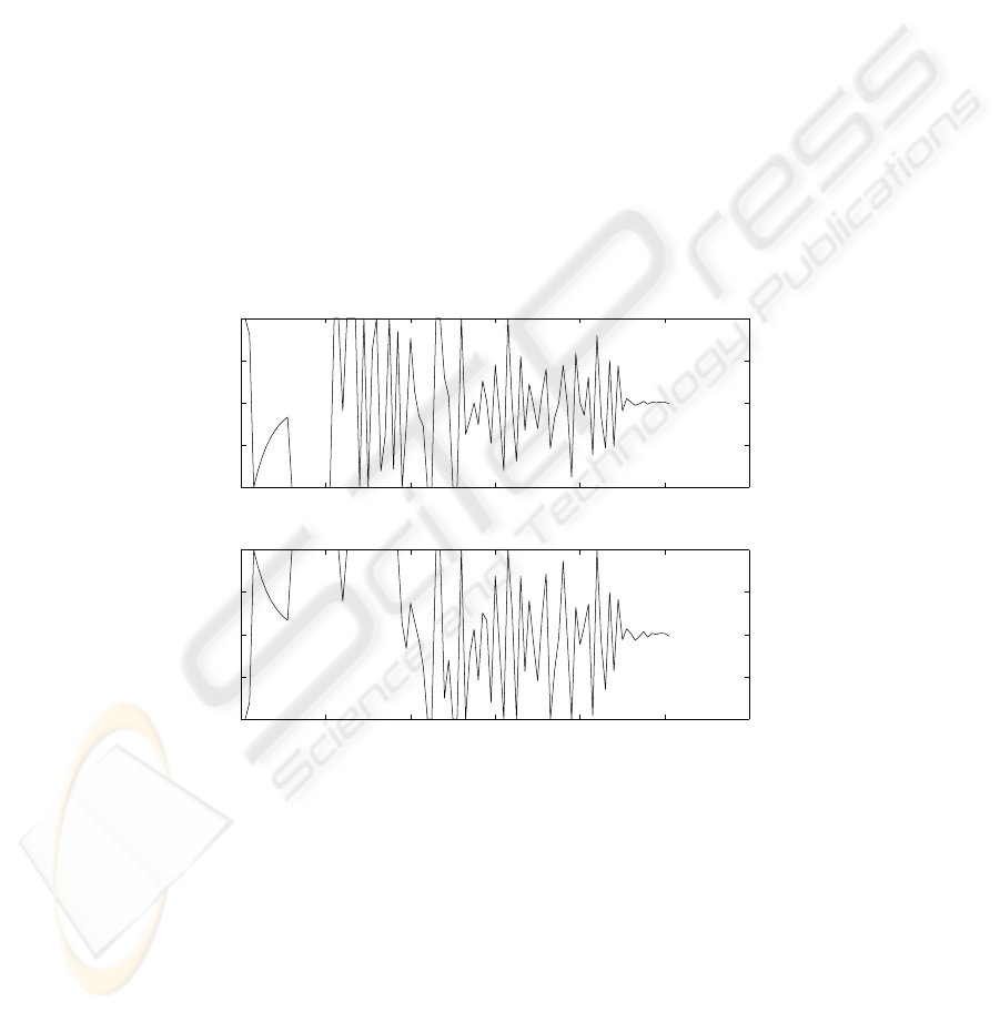
0 20 40 60 80 100 120

−20

−10

0 20 40 60 80 100 120

−20

−10

Fig.1. Velocity components V

and V

in the X

and X

directions. The constraint on the maxi-

mum speed is apparent.

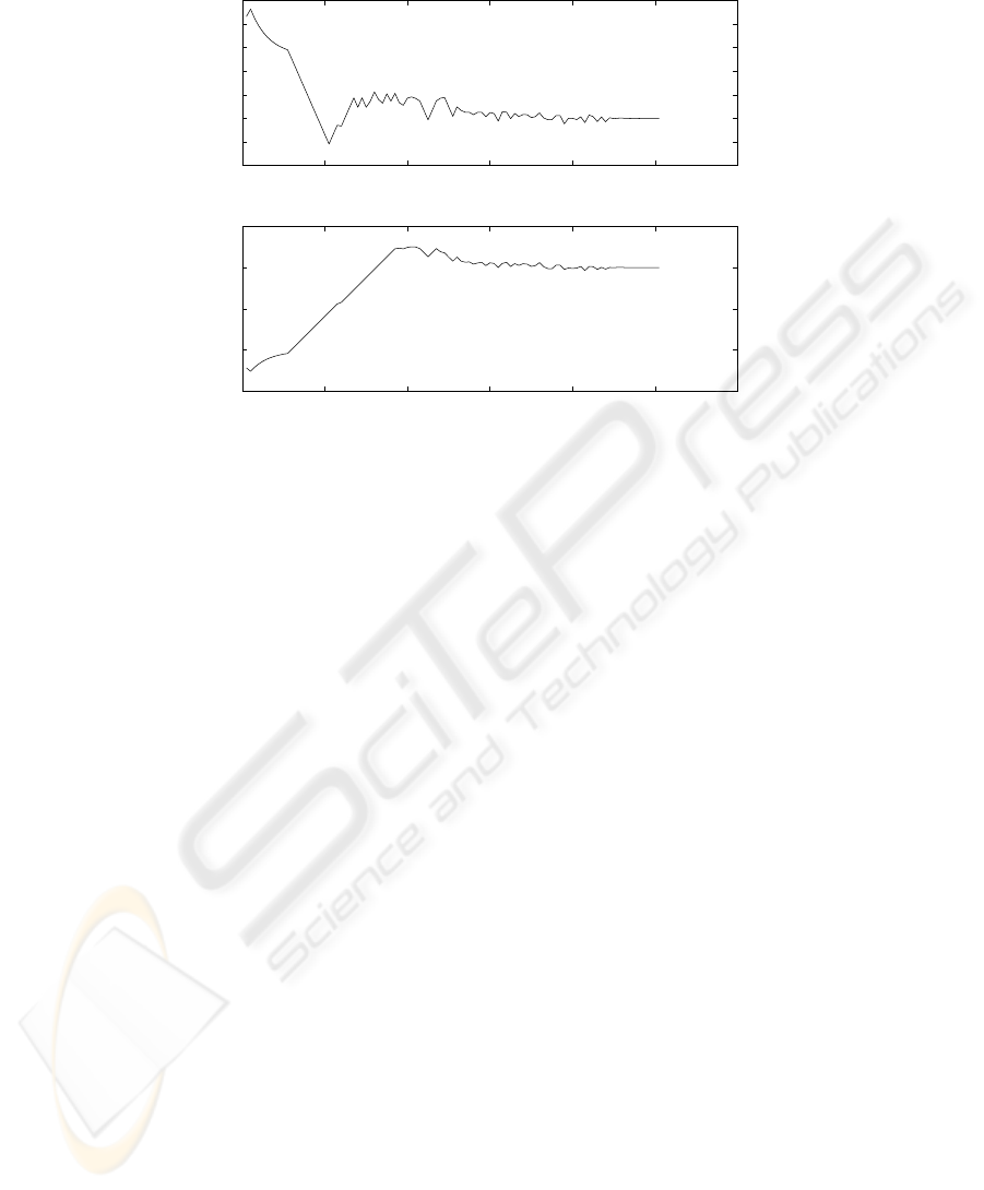
0 20 40 60 80 100 120

100

150

200

250

300

350

400

450

0 20 40 60 80 100 120

−400

−200

200

400

Fig.2. Coordinates of the best trajectory X

and X

as a function of the event counter k. Levy

ﬂights are followed by sticking random walks.

4 Collaborative Search In A 3-D Domain

Here we consider a more difﬁcult search problem, in which the swarm of robots is per-

forming a search for the minimum of a scalar function of three real variables. In the con-

text of autonomous underwater vehicles, the task here is to ﬁnd a minimum temperature

or maximum concentration of a chemical or biological species in a three-dimensional

domain. The number of robots is limited to 10. We select a 3-D test function taken from

the literature, for example the Levy No.8 function [10]. Consider a three-dimensional

body of water with sides 1000 m by 1000 m by 1000 m deep. Select the origin of a carte-

sian system of coordinates in the center of this cube, such that the domain is deﬁned

by:

∈ [X

1min

, X

1max

] = [−500, 500]

∈ [X

2min

, X

2max

] = [−500, 500]

∈ [X

3min

, X

3max

] = [−500, 500] (4.1)

The Levy No.8 function is deﬁned by

f(X

, X

) = sin

(πy

) + f

, y

) + (y

− 1)

(4.2)

, y

) = (y

− 1)

(1 + 10sin

(πy

))

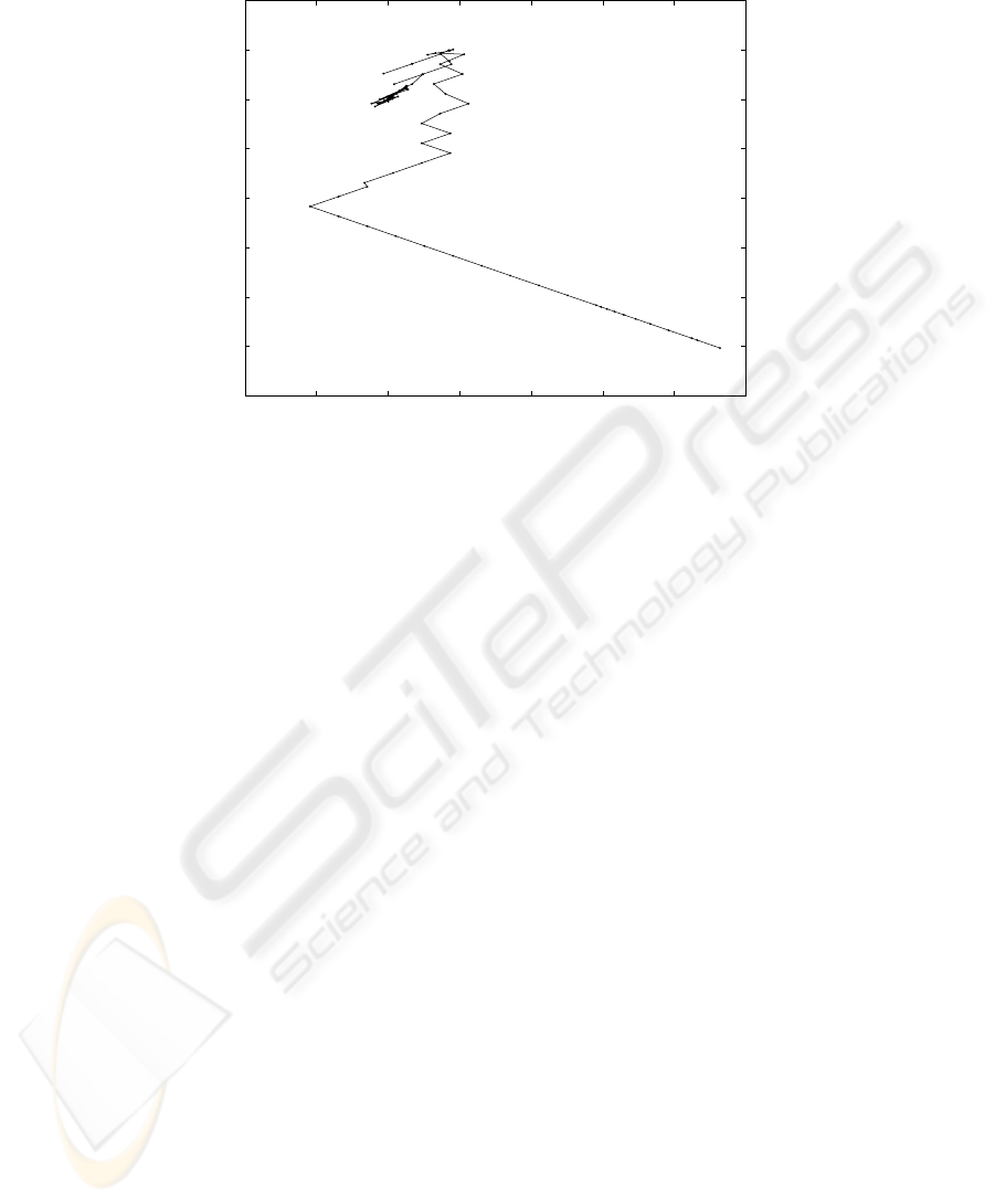
100 150 200 250 300 350 400 450

−400

−300

−200

−100

100

200

300

400

Fig.3. Same trajectory as in Fig.2 with the starting point at the lower right corner and the end

point at the minimum (200,200). Notice the Levy ﬂights along straight line segments and random

short walks around the minimum.

, y

) = (y

− 1)

(1 + 10sin

(πy

)) (4.3)

= 1 + (x

− 1)/4

= 1 + (x

− 1)/4

= 1 + (x

− 1)/4 (4.4)

and the coordinates x

, x

are scaled by a length d = 50 m:

= X

/d, x

= X

/d, x

= X

/d (4.5)

The results are for a delay of τ = 20TU= 500s and the number of autonomous

robot vehicles is N

= 10. The other parameters appearing in the equations of motion

are the same as in the previous case of a 2-D function. The results of a simulation of

the group of robots collaboratively searching for the minimum of the function of three

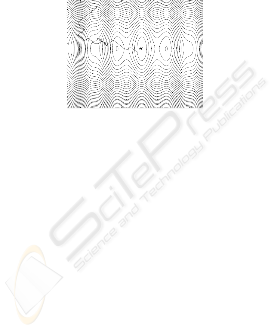
variables are given in Figs. 4-6. The three velocity components are shown in Fig.4.

The constraint on the absolute values of the velocity components is active along some

segments of the motion. The three coordinates as a function of the event counter k are

given in Fig.5. Again there are segments of long Levy ﬂights at maximum speed along

straight lines and segments where the robot performs a random walk in a limited area.

The trajectory is shown in Fig.6 together with a contour plot of the projection of the

f(X

) function on the plane X

=50. The minimum is located at (50,50,50). In

the trajectory projection, it can be seen that segments of long Levy ﬂights are followed

by sticking random walks in the vicinity of the minimum.

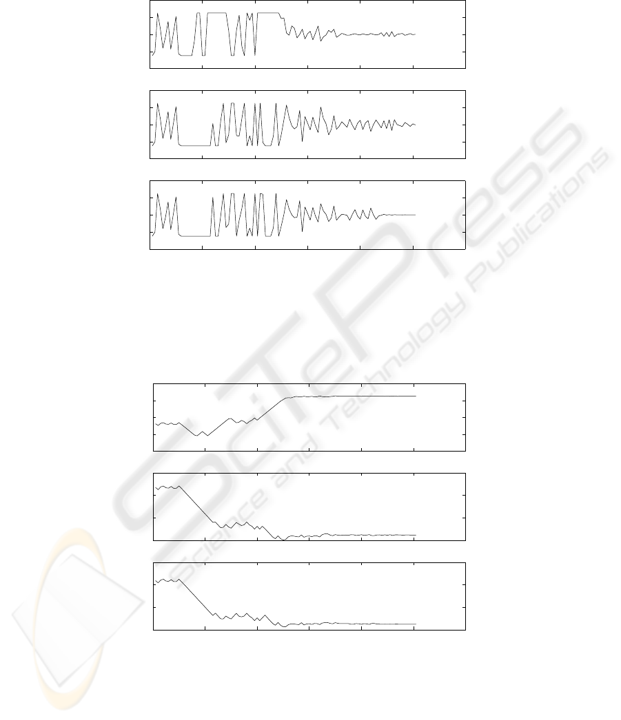
0 20 40 60 80 100 120

−40

−20

0 20 40 60 80 100 120

−40

−20

0 20 40 60 80 100 120

−40

−20

Fig.4. Velocity components V

, V

and V

in the X

, X

and X

directions. The constraint on

maximum speed is apparent.

0 20 40 60 80 100 120

−600

−400

−200

200

0 20 40 60 80 100 120

200

400

600

0 20 40 60 80 100 120

200

400

600

Fig.5. Coordinates of the best trajectory X

, X

and X

as a function of the event counter k. Long

Levy ﬂights are followed by sticking random walks in the vicinity of the minimum.

−500 −400 −300 −200 −100 0 100 200 300 400 500

−500

−400

−300

−200

−100

100

200

300

400

500

Fig.6. Contour plot of the projection of f(X

) on the plane X

=50, with the trajectory of

one robot. The minimum is located at (50,50,50).

5 Conclusion

A method for the cooperative control of a group of robots based on a stochastic model

of swarm intelligen ce has been developed. The network of mobile robots is modeled

by a particle swarm moving randomly in the search domain with the global motion

of the swarm directed and controlled by a central unit which can be a leader robot

or a central server. The method takes into account time delays in the robots network

communications. The motion of each robot in the swarm is governed by a system of two

delay-difference equations. The best solution found collectively by the swarm serves as

the control signal for the network of robots. The control signal can be time delayed due

to communication failure with a subset of the robots in the swarm or due to noise or

attenuation in any of the communication channels. The method was used to solve the

basic problem of collaborative search and optimization in a 2-D and in a 3-D domain. It

was found that the swarm can ﬁnd the optimum despite long time delays in the network

communications.

An unexpected result that was obtained is that the robots trajectories exhibit anom-

alous diffusion, performing long distance Levy ﬂights along straight lines, followed by

sticking random walks in a limited area of the domain, especially when the motion of

the swarm starts converging to the location of the optimum.

References

1. DeSousa, J., Pereira, F.: On coordinated control strategies for networked dynamic control

systems: an application to auvs. In: Proceedings of the 15th International Symposium of

Mathematical Theory of Networks and Systems. (2002)

2. Sperazon, A.: On Control Under Com-munication Constraints in Autonomous Multi-Robot

Systems. Licentiate Thesis, KTH Signals, Sensors and Systems, Royal Institute of Technol-

ogy, Stockholm, Sweden (2004)

3. J. Silva, A. Speranzon, J.D., Johansson, K.: Hierarchical search strategy for a team of au-

tonomous vehicles. In: IFAC. (2004)

4. E. Burian, D. Yoerger, A.B., Singh, H.: Gradient search with autonomous under-water vehi-

cles using scalar measurements. In: IEEE Symposium on Autonomous Underwater Vehicle

Technology, IEEE (1996)

5. Bachmayer, R., Leonard, N.: Vehicle networks for gradient descent in a sampled environ-

ment. In: Proceedings of the 41st IEEE Conference on Decision and Control, IEEE (2002)

6. E. Bonabeau, M.D., Theraulaz, G.: Swarm Intelligence, From Natural to Artiﬁcial Systems.

Santa Fe Institute in the Sciences of Complexity, Oxford University Press, New York (1999)

7. M. Dorigo, G.D., Gambardella, L.: Ant algorithms for discrete optimization. In: Artiﬁcial

Life, Vol.5, pp.137-172 (1999)

8. Eberhart, R., Kennedy, J.: A new optimizer using particle swarm theory. In: Proceedings of

the 6th Symposium on Micro Machine and Human Science, IEEE Service Center (1995)

9. J. Kennedy, R.E., Shi, Y.: Swarm Intelligence. Morgan Kaufman Publishers, San Francisco

(2001)

10. Parsopoulos, K., Vrahatis, M.: Recent approaches to global optimization problems through

particle swarm optimization. In: Natural Computing, Vol.1, pp.235-306, 2002. (2002)

11. T.H. Solomon, E.W., Swinney, H.: Observation of anomalous diffusion and levy ﬂights in a

two-dimensional rotating ﬂow. In: Physical Review Letters, Vol.71, p.3975, APS (1993)

12. T.H. Solomon, E.W., Swinney, H.: Chaotic advection in a two-dimensional ﬂow: Levy ﬂights

and anomalous diffusion. In: Physica D, 76,pp.70-84. (1994)

13. E.R. Weeks, J.U., Swinney, H.: Anomalous diffusion in asymmetric random walks with a

quasi-geostrophic ﬂow example. In: Physica D, 97, pp.291-310. (1996)

14. Weeks, E., Swinney, H.: Anomalous diffusion resulting from strongly asymmetric random

walks. In: Physical Review E, 57, 5, pp.4915-4920, APS (1998)

15. M.F. Schlesinger, G.Z., (eds), U.F.: Levy Flights and Related Topics in Physics. Springer-

Verlag, Berlin (1995)