
Predicting the State of Agents Using Motion and
Occupancy Grids
David Ball
1
and Gordon Wyeth
1
1
School of Information Technology and Electrical Engineering, The University of
Queensland, Australia
Abstract. This paper presents an approach to predicting the future state of dy-
namic agents using an extension to occupancy grids that we have called motion
and occupancy grids. These grids capture both the location and motion of an
agent. The basis of the prediction is to model the behaviour of an agent as the
probability of transitions between the states represented in the grid. Prediction
can then be made using a Markov chain. The potential state explosion inherent
in this method is overcome by dynamically building the state transition matrix
in a tree structure. The results show that the system is able to rapidly develop
probabilistic models of complex agents and predict their future state.
1 Introduction
Autonomous systems have the potential to improve their effectiveness by modifying
their behaviour to adapt to the environment. One resource that would be of use is a
prediction of the future state of the dynamic elements in the environment. There has
been significant successful work in regard to modelling static elements. This paper
explores the more difficult problem of modelling dynamic agents and how to predict
their future state. These predictions are to be used to improve the performance of a
system over time. The key to predicting the motion of an agent is to look for patterns
and tendencies in its behaviour and to be able to model these in an appropriate form
for prediction. This research is targeted at domains where the static features of the
environment are relatively simple, but the dynamic features of the environment form
the greatest obstacles to success.
The agent modelling and prediction approach detailed in the paper is intended to
be part of a larger adaptive system [1] that will enable agents to improve their per-
formance against other agents. This architecture has three steps; classify the behav-
iour of the moving elements of the environment using predefined models, produce
models and predict the behaviour of the moving elements for each class, and exploit
by integrating the models and predictions into the existing planning system to im-
prove its effectiveness. This paper addresses the second step – modelling and predict-
ing the behaviour of moving elements.
The approach is to model the behaviour of an agent’s motion in a discrete form us-
ing a motion and occupancy grid where the connections between states are repre-
sented using a probabilistic state transition matrix. Using the Markov assumption, the
future state is predicted using the state transition matrix and the current state. With
Ball D. and Wyeth G. (2005).
Predicting the State of Agents Using Motion and Occupancy Grids.
In Proceedings of the 1st International Workshop on Multi-Agent Robotic Systems, pages 112-121
DOI: 10.5220/0001192301120121
Copyright
c
SciTePress

the motion and occupancy grid method the state vector and the state transition matrix
can be large. This paper presents a method where the state transition matrix is repre-
sented by a dynamically built tree that is efficient to search and use.
The paper is structured as follows. The following section provides relevant back-
ground and presents existing approaches to agent behaviour prediction. Section three
describes the modelling and prediction system. Section four describes the experimen-
tal setup. Section five presents the results of the experiments and discusses them.
Section six presents early work with using the predictions to adapt the behaviour of
an agent. Lastly section seven concludes the paper.
2 Background
This section provides background on the Markov approach to modelling and predict-
ing the future behaviour for agents. It also briefly describes the occupancy grids that
form the basis of the motion and occupancy grids used in this work.
2.1 Markov Chains
A process is said to be Markov if the future state distribution depends only on the
present state, in other words, the future is conditionally independent of the past. A
Markov Chain consists of a finite number of states and a state transition matrix which
contains probabilities of moving between states [2]. So:
)|(),...,,|(
11111100 −−−−
=
=
=
=
=
==
tttttt
iXjXPiXiXiXjXP
(1)
The state of the process can therefore be predicted forward t time steps by multi-
plying the state transition matrix t times. So if X represents the state of the process
and A is the state transition matrix (a stochastic matrix) then to predict the state for-
ward one time step:
tt
XAX
⋅
=
+1
(2)
If there are n states in X then A is of size n × n.
The Markov assumption allows for simple state transition model approaches but
predictions cannot be guaranteed if the assumption is invalid. Typically as the
agent’s architecture becomes more reactive (and hence carries less internal state) a
Markov predictor will increase its performance. Predicting the future state using
Markov Chains is not new. Improvements such as semi-Markov processes (SMP) [2]
have allowed arbitrary state duration and the augmented Markov Models (AMM) [3]
that allows additional statistics in links and nodes so that it can restructure a model.
The AMM is dynamically constructed by adding state nodes as the agent enters pre-
viously unseen states. This differs from the method in this paper where the entire state
is predefined and the state transition matrix is dynamically built. This is useful where
the state space is large as it can be implemented for efficient searching.
2.2 Occupancy Grids
The occupancy grid method [4, 5] provides a probabilistic approach to representing
how a region of space is occupied. It has been successfully used for representing
obstacles for robot navigation. The method does not capture the motion of the obsta-
cles. The method in this paper extends this method so that it can capture and represent
the motion of occupied space or in this case, dynamic agents.
3 Prediction Approach
This section describes the extensions to an occupancy grid required to deal with mov-
ing elements. It explains the problem of state explosion inherent in this method and
how it can be addressed using dynamic state transition trees.
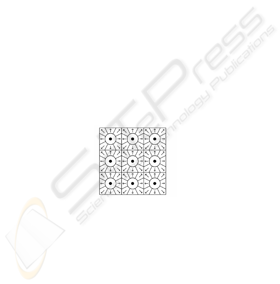
3.1 Motion and Occupancy Grid Method
Fig. 1 shows a representation of the motion and occupancy grid cells. The occupancy
grid is suitable for representing the probability distribution of the future occupied
space for an agent. The environment is divided into grid cells that represent the agent
occupying particular locations. The future state of the agent can be predicted by de-
termining the probability of transitioning between grid cell states. However, this ig-
nores the agent’s motion within the grid cell and different paths the agent may take
through the same grid cell.
Fig. 1. This figure shows how the state of an agent is represented using the motion and occu-
pancy grid. The centre circle represents stationary (the robot staying in same grid cell) and the
cells surrounding the circle represent the possible directions of motion.
The motion grid captures the agent’s current direction of motion (also referred to
as its heading direction) so that it can distinguish between different motion types
through the grid cell. For example, an agent may have two motion paths through a
cell, one from bottom to top and the other from left to right. If the motion of an agent
is not captured the probability distribution will show the predicted motion to the right
and the top. The motion grid allows for the prediction for the two motion types
through the cell to be separated. The centre circle represents an agent that is station-

ary which is an agent that will maintain the same occupancy grid state. The other
cells represent directions of motion for the agent, dividing the domain of possible
directions into equal amounts.
Motion and occupancy grids are fully connected between states, so that each state
has probabilities associated with transitioning to all other states, even if they are zero.
The state transition probabilities are histogram based. The probability update equation
is:
1
1],[
],[
1
1
+
+
×
=
+
+
Xt
Xtttcurrent
ttnew
c
cXXA
XXA
(3)
A[X
t
, X
t+1
] is the element in the state transition matrix that represents the probabil-
ity of transitioning from state X
t
to X
t+1
. c
Xt
is the count of the number of times the
state X
t
has been initial state in a transition. To decrease computation time, the num-
ber of transitions between each state is recorded c
Xt->Xt+1
and so the probability update
equation becomes:
1
1
],[
1
1
+
+
=
+>−
+
Xt
XtXt
ttnew
C
C
XXA
(4)
3.2 Extending the State Vector
Typically an agent’s choice of action is dependent on other agents or other dynamic
features of the environment. For the Markov assumption to hold true, these features
must also be represented in the state vector. This dramatically increases the size of the
state transition matrix. If the predicted agent’s behaviour is dependent on the behav-
iour of another agent, then the state vector would hold not only the predicted agent’s
occupancy and motion grid, but also that of the other agent.
A motion and occupancy grid state vector has four state variables {x, y, v
x
, v
y
}. In
the testing environment in this paper the x direction is divided into 15 columns and
the y direction into 12 rows. Velocity is coarsely binned as being left, stationary or
right for v
x
, and up, stationary or down for v
y
. Consequently there are a total of 15 ×
12 × 3 × 3 = 1620 states that represent the position and motion of the agent. If the
agent is dependent on a dynamic element that uses the same motion and occupancy
grid this becomes 2,624,400 states to represent the two agents.
The state transition matrix is in a squared relationship to the size of the state vec-
tor. As the state vector increases the required number of bytes for a fully defined state
transition matrix quickly becomes larger that is possible to store in physical memory.
Not only can the state transition matrix be too large to store on a typical PC but also
multiplying all the entries (for prediction) can have a large computational cost.
3.3 Dynamic Tree State Transition Matrix
To overcome the limitation associated with the typically large motion and occupancy
grids this approach dynamically populates the state transition matrix. Each new entry
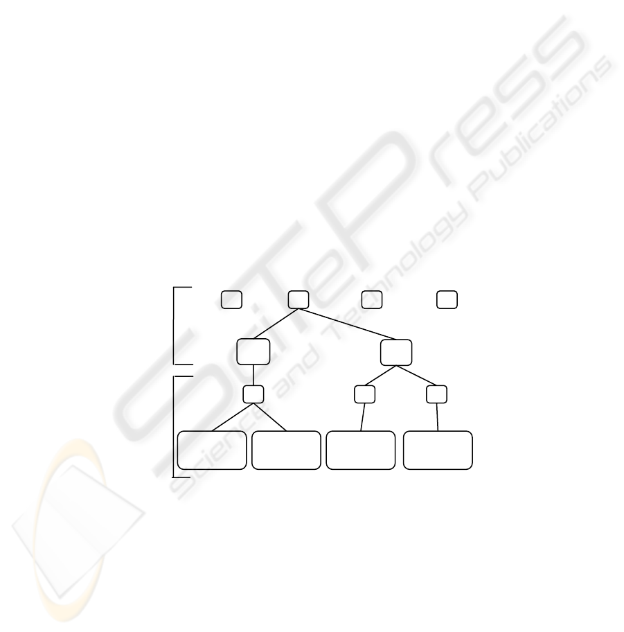
increases the size of the state transition matrix in memory in a linear fashion. A
straightforward approach to populating the matrix would be to dynamically build a
one dimensional list where previously unseen entries are added. However, this would
not be computationally effective as the entire array would need to be searched to
determine if an entry was new. Also, during the prediction phase, the entire array
would need to be searched to find corresponding entries in the state matrix.
This papers approach uses a dynamically constructed tree to represent the state
transition matrix. Each level of the tree represents an index to the state vector based
on one of the state variables. For example, consider the simplified case of an occu-
pancy grid where the grid may be indexed by the x and y variables representing the
location of an agent.
The state transition tree for this agent is shown in Fig. 2. The first level of the tree
represents the x index for all locations the agent has visited so far. As the agent visits
new columns, new x nodes will be created at this level. The second level is indexed
on the y location, again only creating nodes as the agent visits new rows in the grid.
Each node in this level stores the number of times this node has been visited for the
probability update equation (Equation 4). The tree structure is then repeated below to
show the transition probabilities to other grid cells. Again, storage elements are only
created as needed, with the lowest layer of the tree storing the probability of the tran-
sition A[X
t
, X
t+1
] as well as the count of the number of transitions between states C
Xt-
>Xt+1
.
A tree is also dynamically constructed to store the predictions for each time step.
This allows for the state of the agent to be predicted forward computationally effec-
tively. This tree contains branches to represent all states that have been the results of
a transition. This tree has half as many levels as the state transition tree.
Fig. 2. The state transition tree represents the state transition matrix and is dynamically built.
Each level of the tree represents a vector of state variables. The depth is fixed and the prob-
abilities are stored in the lowest level of the tree. Except for the probability layer the nodes
(shown as white squares) contain pointers to variables within the next layers state vector. This
tree is a two state vector tree but the tree can be any even number of levels. The number of
transitions from each state is recorded where it branches from the current state to the next state.
Current
State
Next
State
x
t
x
t+1
y
t
y
t+1
A
[(2,3),(2,1)]
c
(2,3) -> (2,1)
c
(2,3)
c
(2,4)
2
3
43
4
22
4
4
1 4 5
1
A
[(2,3),(2,4)]
c
(2,3) -> (2,4)
A
[(2,4),(2,4)]
c
(2,4) -> (2,4)
A
[(2,4),(4,5)]
c
(2,4) -> (4,5)

4 Experimental Setup
This section describes the testing environment and experimental setup to the test the
performance of the proposed prediction system.
The testing environment is the RoboCup Small Size League [6] and the research
platform is the RoboRoos. In this league both teams have five robots. The rules are
similar to the human version of the game (FIFA). There are two 10 minute halves.
The robots are fully autonomous in the sense that no strategy or control input is al-
lowed by the human operators during play.
The prediction method is tested within the existing robot soccer system. The simu-
lator simulates two teams of robots in line with the 2003 RoboCup Small Size League
rules and regulations. This includes simulating some of the important human referee
tasks such detection of when a goal is scored and restarting play. The simulator has a
very high fidelity with a one millisecond resolution in the simulation of all robot and
ball kinematics, dynamics and collisions. It closely simulates the performance of the
real robots. The vision and intelligence systems are simulated at 60 Hz. Simulations
including the prediction algorithm ran faster than real time on a Pentium-M laptop
computer. The time between the current and next state, one time step, is 250 millisec-
onds (15 frames). The model is updated at every visual update (60 Hz). The agents
are predicted every 83.3 milliseconds which is 5 frames. The agents are predicted
forward 1 second into the future (a significant time in robot soccer) representing 4
steps in the Markov chain. At the agent’s top speed of 1.5 metres/second they can
move approximately 8 grid squares in the predicted time.
The field is divided up so that each occupancy grid cell is approximately the same
size as an agent. This gives 15 x 12 grid squares. The current heading direction is
broken into 8 directions and stationary to form the motion grid. This is converted into
a 3 x 3 matrix where the centre cell (1,1) is for stationary and the other cells hold
appropriate heading directions. An agent is classified as stationary if its velocity is
below a threshold. This threshold is the velocity where an agent is just as likely to
maintain its current occupancy state as it is to change state. This is half of the cell
width divided by the time step time. This gives a threshold velocity of 0.36 me-
tres/second. When the system is unable to make a prediction (the agent is in a previ-
ously unseen state) the system predicts that the agent will continue with its current
motion. If the agent is stationary then it is predicted to maintain its current location.
The system was tested in three different situations of increasing difficulty.
• Figure of Eight Path – This involved an agent tracing out a figure of eight path.
This has no relationship to robot soccer but is used to demonstrate the approach.
• Goal Shooting - This involved one agent interacting with a ball against five oppo-
sition agents that were held stationary in a defensive formation. The player’s ac-
tions were to acquire, move and kick the ball into the opponent’s goal. Results
were recorded for a state transition tree that modelled the dependency on the mo-
tion of the ball and one that doesn’t. This experiment lasted for twenty minutes.
• Full Game – This was a normal game lasting twenty minutes with most of the
rules of the SSL. This is the most difficult domain for the predictor. Each player on
the opposing team was modelled and predicted relative to the motion of the ball.
5 Results
This section first demonstrates the proper operation of the system and highlights an
important benefit of the motion grid. Next the results comparing the predicted and
actual positions are presented and discussed.
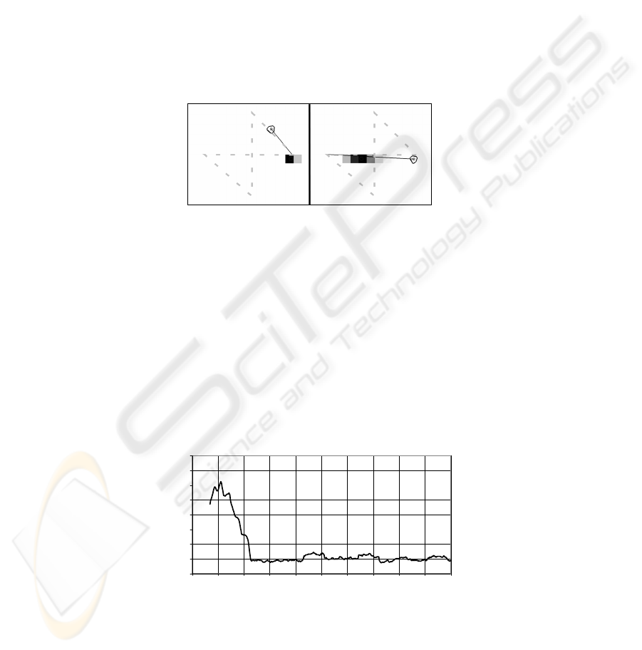
Two instances of the agent following the figure of eight path and its predicted fu-
ture probability distribution are shown in Fig. 3. The time between the left figure and
the right figure is equal t the prediction time (1 second), which demonstrates that the
system predicted accurately in this simple case. The right-hand diagram in the figure
demonstrates an important ability of this approach. The agent’s state has been pre-
dicted correctly through the intersection of the figure eight. This is only possible
because the agent’s motion is modelled along with its position. In a system where
only the occupancy is modelled the probability distribution would extend in two di-
rections, left and up.
Fig. 3. This figure shows the agent and its predicted probability distribution for two instances
of the agent traversing the figure of eight path. The path is shown as a dashed line and the
agent is represented by the polygon. The line from the agent shows its current navigation
command. The darkened grid cells show the prediction of the agent’s position, with a darker
cell representing a greater likelihood.
Fig. 4 shows the quantitative results for the figure of eight experiment, comparing
the predicted position of the agent with its true position after the prediction time has
elapsed. The predicted position is a weighted average of the probability distribution
that represents the future occupancy of an agent. The error is the Euclidean distance
between the centres of the predicted and the true cell. The error rapidly decreases
after one complete cycle is made. After two cycles the error stabilises at approxi-
mately half a grid cell representing the quantisation noise of the grid system.
Prediction Error for the Figure of Eight Experiment
0
0.5
1
1.5
2
2.5
3
3.5
4
10 15 20 25 30 35 40 45 50 55 60
Time (Seconds)
Error (Grid Cells)
Fig. 4. Figure of Eight prediction error. The error rapidly decreases after the agent has started
the second cycle and by the third the error has stabilised at approximately half a grid cell.
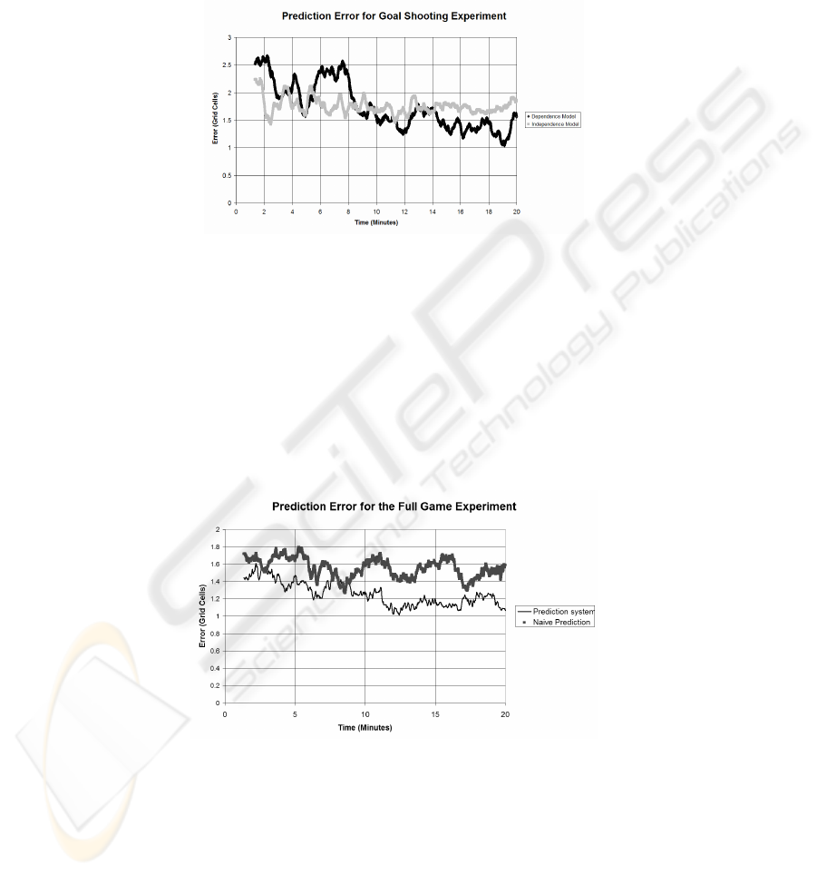
Fig. 5 shows the prediction error for the Goal Shooting experiment. In the experi-
ment where the agent’s motion is assumed to be independent from the motion of the
ball, the error is generally constant. In the experiment where dependence on the ball
is assumed the error drops through the experiment, ending with a lower average error
than the independence experiment. This demonstrates the importance of modelling
the relationship between dynamic elements when there is a dependence relationship.
Fig. 5. Goal Shooting prediction error. The upper error line shows the effect of assuming that
the prediction is independent of the ball’s motion. A simple, but not very accurate, model of
the motion is quickly learnt. When the ball’s motion is included in the state vector, the learning
is a little slower, but the end result is more accurate.
The ability to predict the motion of opposing agents in a game of robot soccer is a
highly challenging task. Fig. 6 shows the results for the prediction system when com-
pared to a naïve predictor that assumes that the robot will continue move in the same
direction if it is moving or will remain still if it is currently still. This graph shows
that the prediction system consistently outperforms the naïve predictor, with steadily
improving performance through out the match.
Fig. 6. Full Game prediction error. This graph compares the error naively assuming constant
motion with the prediction system error. This shows the prediction systems error decreasing
throughout the experiment.
These results demonstrate that the prediction approach is able to learn and predict the
opponent’s motion. In the Figure of Eight experiment the model size stabilises at
approximately 30 Kilobytes. The Goal Shooting experiment model reaches a size of
4.8 Megabytes and the Full Game experiment model reaches a size of 12.2 Mega-
bytes. These storage sizes are significantly less than for a fully defined state transition
matrix. The models were still significantly growing at the end of the Goal Shooting
and Full Game experiments indicating that the agents were still traversing previously
unseen states. Potentially the error would continue to decrease if the experiments
were run for a longer period of time.
6 Applying the Predictions
While the above results are a measure of the quality of the predictions, they do not
reflect one of the strengths of this approach. The prediction process ends with a prob-
ability distribution representing the agent’s most likely future occupancy as shown in
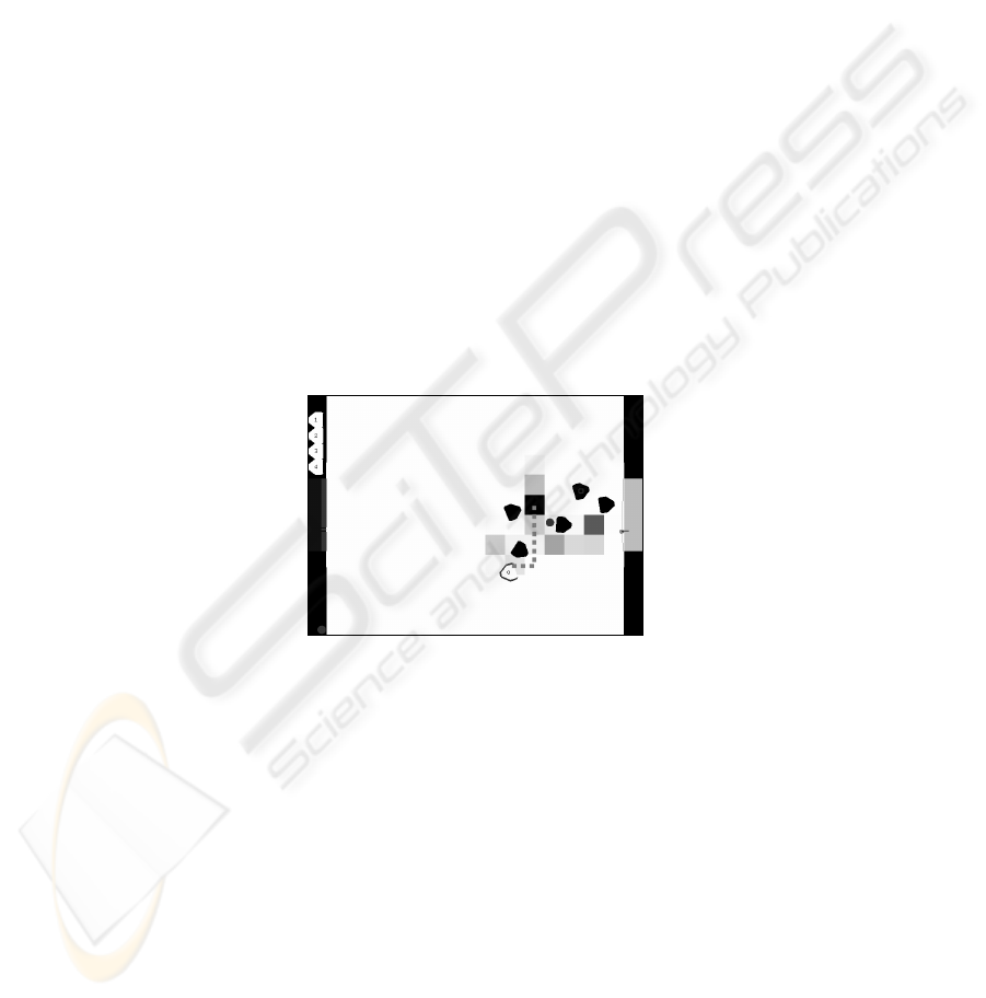
Fig. 7. This probability distribution is an example from the Goal Shooting experiment
and is just after the ball has been kicked at the opponent’s goal. The grey dotted path
shows the agent’s actual path during the predicted time. Interpreting the distribution,
the agent is most likely to travel from its current position along the dotted path but
may also travel towards the opponent’s goal. There is also a small probability of the
agent maintaining its current position. Measuring the weighted average to the actual
position (as was done in the results in Section 5) does not reflect the usefulness of
knowing the shape of the likely paths that the agent will take. This can only be as-
sessed by exploiting the predictions.
Fig. 7. Typical prediction probability distribution. The darker square cells represent a higher
probability value. There are five opponent agents. The dotted grey line shows the agents mo-
tion during the predicted time. This figure demonstrates a strength of this approach that is not
reflected in the Euclidean distance error results.
The predictions were applied to improving the ability of the agents to score goals.
In robot soccer, one of the important choices for the planner is to determine the loca-
tion that is the best for scoring goals. The MAPS planner [7] used by the RoboRoos
considers the current position of the opposing agents and the clear paths to goal when
choosing a shooting location. Instead of treating the opponents as crisp positions, the
probability distributions developed from the predictions of opposing agents were
used.
When using offence strategies involving passing to the shooting player, or creating
opportunities for the shooting player to move into space the adapting team was more

likely to win the game. However, when using strategies that were designed to disrupt
the defence to create goal scoring opportunities the adapting team was more likely to
lose the game. This initial exploitation work has raised the following issues:
• The choice of overall strategy to combine with the predictions is important. For
example using strategies designed to disrupt the regular motion of the agents under
prediction will cause poor modelling and prediction performance.
• There is an inconsistency in basing the choice of action on a prediction that will be
invalid if the choice of action does not lead to the prediction.
• While the opponents may not be adapting their strategy using an agent model, their
motion is likely to change as the choice of action of the predicting agent changes.
7 Conclusion
This paper has presented an approach to predicting the future state of agents using
motion and occupancy grids and the Markov Chain method. It was shown that this
method is able to separate different motion paths. A method of storing the typically
large state transition matrices by dynamically building a tree representation was pre-
sented that enables the typically large state spaces. The results demonstrate that the
approach is able to separate different motion paths and they show the importance of
modelling the agent’s dependencies. The error from the prediction system decreases
as the experiments continue. Future work will further explore methods of using the
predictions to improve the performance of an autonomous planning system.
References
1. Ball, D. and G. Wyeth. Modeling and Exploiting Behavior Patterns in Dynamic Environ-
ments. in 2004 IEEE/RSJ International Conference on Intelligent Robots and Systems
(IROS). 2004. Sendai, Japan.
2. Ross, S.M., Applied Probability Models with Optimization Applications. 1992, New York:
Dover Publications, Inc.
3. Goldberg, D. and M.J. Mataric. Reward Maximization in a Non-Stationary Mobile Robot
Environment. in The Fourth International Conference on Autonomous Agents. 2000. Barce-
lona, Spain.
4. Elfes, A.E. Occupancy grids: A stochastic spatial representation for active robot perception.
in Sixth Conference on Uncertainty in AI. 1990.
5. Moravec, H.P. and A.E. Elfes. High resolution maps from wide angle sonar. in Proceedings
of the 1985 IEEE International Conference on Robotics and Automation. 1985. Washington,
D.C, USA.
6. Kitano, H., et al. RoboCup: The Robot World Cup Initiative. in IJCAI-95 Workshop on
Entertainment and AI/ALife. 1995.
7. Ball, D. and G. Wyeth. Multi-Robot Control in Highly Dynamic, Competitive Environ-
ments. in RoboCup 2003. 2003. Padua, Italy: Springer Verlag.
