
DIRECT GRADIENT-BASED REINFORCEMENT LEARNING
FOR ROBOT BEHAVIOR LEARNING
Andres El-Fakdi, Marc Carreras and Pere Ridao
Institute of Informatics and Applications, University of Girona, Politecnica 4, Campus Montilivi, 17071 Girona, Spain
Keywords: Robot Learning, Autonomous robots.
Abstract: Autonomous Underwater Vehicles (AUV) represent a challenging control problem with complex, noisy,
dynamics. Nowadays, not only the continuous scientific advances in underwater robotics but the increasing
number of sub sea missions and its complexity ask for an automatization of submarine processes. This paper
proposes a high-level control system for solving the action selection problem of an autonomous robot. The
system is characterized by the use of Reinforcement Learning Direct Policy Search methods (RLDPS) for
learning the internal state/action mapping of some behaviors. We demonstrate its feasibility with simulated
experiments using the model of our underwater robot URIS in a target following task.
1 INTRODUCTION
A commonly used methodology in robot learning is
Reinforcement Learning (RL) (Sutton, 1998). In RL,
an agent tries to maximize a scalar evaluation
(reward or punishment) obtained as a result of its
interaction with the environment. The goal of a RL
system is to find an optimal policy which maps the
state of the environment to an action which in turn
will maximize the accumulated future rewards. Most
RL techniques are based on Finite Markov Decision
Processes (FMDP) causing finite state and action
spaces. The main advantage of RL is that it does not
use any knowledge database, so the learner is not
told what to do as occurs in most forms of machine
learning, but instead must discover actions yield the
most reward by trying them. Therefore, this class of
learning is suitable for online robot learning. The
main disadvantages are a long convergence time and
the lack of generalization among continuous
variables.
In order to solve such problems, most of RL
applications require the use of generalizing function
approximators such artificial neural-networks
(ANNs), instance-based methods or decision-trees.
As a result, many RL-based control systems have
been applied to robotics over the past decade. In
(Smart and Kaelbling, 2000), an instance-based
learning algorithm was applied to a real robot in a
corridor-following task. For the same task, in
(Hernandez and Mahadevan, 2000) a hierarchical
memory-based RL was proposed.
The dominant approach has been the value-
function approach, and although it has demonstrated
to work well in many applications, it has several
limitations, too. If the state-space is not completely
observable (POMDP), small changes in the
estimated value of an action cause it to be, or not be,
selected; and this will detonate in convergence
problems (Bertsekas and Tsitsiklis, 1996).
Over the past few years, studies have shown that
approximating directly a policy can be easier than
working with value functions, and better results can
be obtained (Sutton et al., 2000) (Anderson, 2000).
Instead of approximating a value function, new
methodologies approximate a policy using an
independent function approximator with its own
parameters, trying to maximize the expected reward.
Examples of direct policy methods are the
REINFORCE algorithm (Williams, 1992), the
direct-gradient algorithm (Baxter and Bartlett, 2000)
and certain variants of the actor-critic framework
(Konda and Tsitsiklis, 2003). Some direct policy
search methodologies have achieved good practical
results. Applications to autonomous helicopter flight
(Bagnell and Schneider, 2001), optimization of robot
locomotion movements (Kohl and Stone, 2004) and
robot weightlifting task (Rosenstein and Barto,
2001) are some examples.
The advantages of policy methods against value-
function based methods are various. A problem for
which the policy is easier to represent should be
solved using policy algorithms (Anderson, 2000).
Working this way should represent a decrease in the
225
El-Fakdi A., Carreras M. and Ridao P. (2005).
DIRECT GRADIENT-BASED REINFORCEMENT LEARNING FOR ROBOT BEHAVIOR LEARNING.
In Proceedings of the Second International Conference on Informatics in Control, Automation and Robotics - Robotics and Automation, pages 225-231
DOI: 10.5220/0001188902250231
Copyright
c
SciTePress

computational complexity and, for learning control
systems which operate in the physical world, the
reduction in time-consuming would be notorious.
Furthermore, learning systems should be designed to
explicitly account for the resulting violations of the
Markov property. Studies have shown that stochastic
policy-only methods can obtain better results when
working in POMDP than those ones obtained with
deterministic value-function methods (Singh et al.,
1994). On the other side, policy methods learn much
more slowly than RL algorithms using value
function (Sutton et al., 2000) and they typically find
only local optima of the expected reward (Meuleau
et al., 2001).
In this paper we propose an on-line direct policy
search algorithm based on Baxter and Bartlett’s
direct-gradient algorithm OLPOMDP (Baxter and
Bartlett, 1999) applied to a real learning control
system in which a simulated model of the AUV
URIS (Ridao et al., 2004) navigates a two-
dimensional world. The policy is represented by a
neural network whose input is a representation of the
state, whose output is action selection probabilities,
and whose weights are the policy parameters. The
proposed method is based on a stochastic gradient
descent with respect to the policy parameter space, it
does not need a model of the environment to be
given and it is incremental, requiring only a constant
amount of computation step. The objective of the
agent is to compute a stochastic policy (Singh et al.,
1994), which assigns a probability over each action.
Results obtained in simulation show the viability of
the algorithm in a real-time system.
The structure of the paper is as follows. In
section II the direct-policy search algorithm is
detailed. In section III a description of all the
elements that affect our problem (the world, the
robot and the controller) are commented. The
simulated experiment description and the results
obtained are included in section IV and finally, some
conclusions and further work are included in section
V.
2 THE RLDPS ALGORITHM
A partially observable Markov decision process
(POMDP) consists of a state space S, an observation
space Y and a control space U. For each state
iS∈
there is a deterministic reward r(i). As
mentioned before, the algorithm applied is designed to
work on-line so at every time step, the learner (our
vehicle) will be given an observation of the state and,
according to the policy followed at that moment, it will
generate a control action. As a result, the learner will be
driven to another state and will receive a reward
associated to this new state. This reward will allow us to
update the controller’s parameters that define the policy
followed at every iteration, resulting in a final policy
considered to be optimal or closer to optimal. The
algorithm procedure is summarized in Table 1.
Table 1: Algorithm: Baxter & Bartlett’s OLPOMDP
1: Given:
•
0T >
• Initial parameter values
0
K
θ
∈
• Arbitrary starting state i
0
2: Set z
0
= 0 ( z
0
K
∈
)
3: for t = 0 to T do
4: Observe state y
t
5: Generate control action u
t
according to current policy
(, )
t
y
µθ
6: Observe the reward obtained r(i
t+1
)
7: Set
8: Set
9: end for
The algorithm works as follows: having
initialized the parameters vector
0
θ
, the initial state
i
0
and the gradient
0
0z
=
, the learning procedure
will be iterated T times. At every iteration, the
parameters gradient
t
z will be updated. According
to the immediate reward received
1
()
t
ri
+
, the new
gradient vector
1t
z
+
and a fixed learning
paramenter
α
, the new paramenter vector
1t
θ
+
can be
calculated. The current policy
t
µ
is directly modified
by the new parameters becoming a new policy
1t
µ
+
that will be followed next iteration, getting
closer, as
tT→
to a final policy
T
µ
that represents a
correct solution of the problem.
In order to clarify the steps taken, the next lines
will relate the update parameter procedure of the
algorithm closely. The controller uses a neural
network as a function approximator that generates a
stochastic policy. Its weights are the policy
parameters that are updated on-line every time step.
The accuracy of the approximation is controlled by
the parameter
[0,1)
β
∈
.
The first step in the weight update procedure is
to compute the ratio:
1
(, )
(, )
t
t
ut
tt
ut
y
zz
y
µ
θ
β
µθ
+
∇
=+
111
()
tt tt
ri z
θ
θα
+
++
=
+
ICINCO 2005 - ROBOTICS AND AUTOMATION
226
(, )
(, )
t
t
ut
ut
y
y
µ
θ
µθ
∇
(1)
for every weight of the network. In AANs like the
one used in the algorithm the expression defined in
step 7 of Table 1 can be rewritten as:
1tttt
zzy
β
δ
+
=+
(2)
At any step time t, the term
t
z represents the
estimated gradient of the reinforcement sum with
respect to the network’s layer weights. In addition,
t
δ
refers to the local gradient associated to a single
neuron of the ANN and it is multiplied by the input
to that neuron
t
y . In order to compute these
gradients, we evaluate the soft-max distribution for
each possible future state exponentiating the real-
valued ANN outputs
{
}
1
,...,
n
oobeing n the number
of neurons of the output layer (Aberdeen
, 2003).
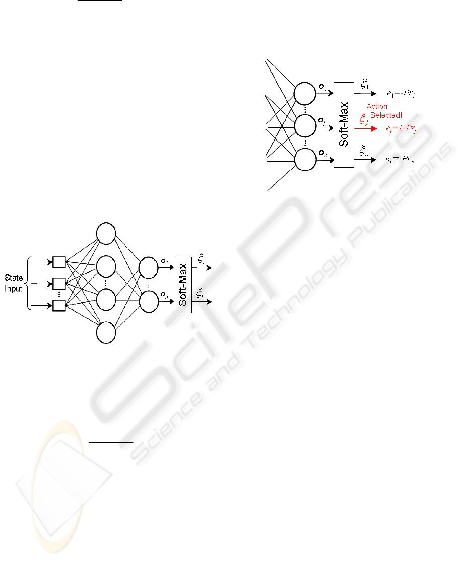
Figure 1: Schema of the ANN architecture used.
After applying the soft-max function, the outputs
of the neural network give a weighting,
(0,1)
j
ξ
∈
to
each of the vehicle’s thrust combinations. Finally,
the probability of the i
th
thrust combination is then
given by:
1
exp( )
Pr
exp( )
i
i
n
z
z
o
o
=
=
∑
(3)
Actions have been labeled with the associated
thrust combination, and they are chosen at random
from this probability distribution.
Once we have computed the output distribution
over the possible control actions, next step is to
calculate the gradient for the action chosen by
applying the chain rule; the whole expression is
implemented similarly to error back propagation
(Haykin
, 1999). Before computing the gradient, the
error on the neurons of the output layer must be
calculated. This error is given by expression (4).
Pr
j
jj
ed
=
−
(4)
The desired output
j
d
will be equal to 1 if the action
selected was
j
o
and 0 otherwise (see Fig. 2).
Figure 2: Soft-Max error computation for every output.
With the soft-max output error calculation
completed, next phase consists in computing the
gradient at the output of the ANN and back
propagate it to the rest of the neurons of the hidden
layers. For a local neuron j located in the output
layer we may express the local gradient for neuron j
as:
'
·()
o
jjjj
eo
δϕ
=
(5)
Where
j
e
is the soft-max error at the output of
neuron j,
'
()
j
j
o
ϕ
corresponds to the derivative of the
activation function associated with that neuron and
j
o is the function signal at the output for that
neuron. So we do not back propagate the gradient of
an error measure, but instead we back propagate the
soft-max gradient of this error. Therefore, for a
neuron j located in a hidden layer the local gradient
is defined as follows:
'
()
h
jjj kkj
k
ow
δϕ δ
=
∑
(6)
When computing the gradient of a hidden-layer
neuron, the previously obtained gradient of the
following layers must be back propagated. In (6) the
term
'
()
j
j
o
ϕ
represents de derivative of the
activation function associated to that neuron,
j
o
is
the function signal at the output for that neuron and
finally the summation term includes the different
gradients of the following neurons back propagated
DIRECT GRADIENT-BASED REINFORCEMENT LEARNING FOR ROBOT BEHAVIOR LEARNING
227
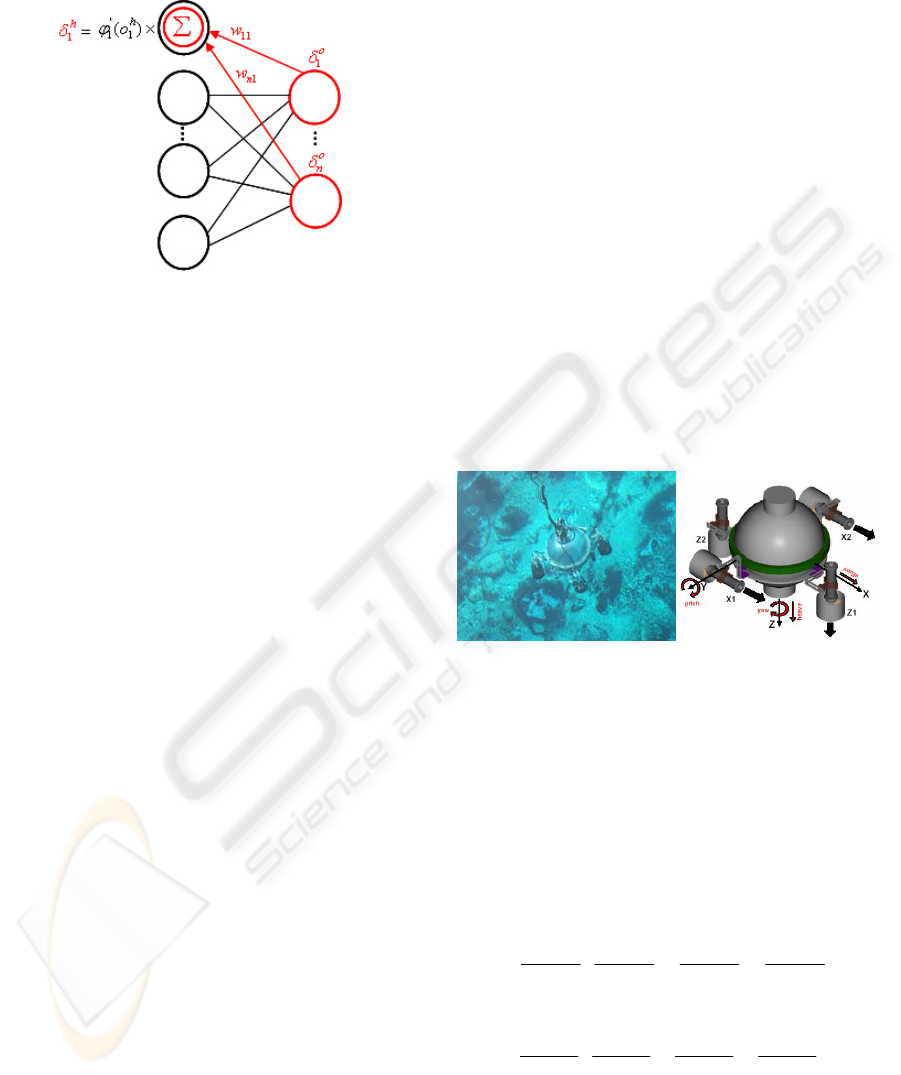
by multiplying each gradient to its corresponding
weighting (see Fig. 3).
Figure 3: Gradient computation for a hidden-layer neuron.
Having all local gradients of the all neurons
calculated, the expression in (2) can be obtained and
finally, the old parameters are updated following the
expression:
111
()
tt tt
ri z
θ
θγ
+++
=+ (7)
The vector of parameters
t
θ
represents the
network weights to be updated,
1
()
t
ri
+
is the reward
given to the learner at every time step,
1t
z
+
describes
the estimated gradients mentioned before and at last
we have
γ
as the learning rate of the RLDPS
algorithm.
3 CASE TO STUDY: TARGET
FOLLOWING
The following lines are going to describe the
different elements that take place in our problem.
First, the simulated world will be detailed, in a
second place we will present the underwater vehicle
URIS and its model used in our simulation. At last, a
description of the neural-network controller is
presented.
3.1 The World
As mentioned before, the problem deals with the
simulated model of the AUV URIS navigating a
two-dimensional world constrained in a plane region
without boundaries. The vehicle can be controlled in
two degrees of freedom (DOFs), surge (X
movement) and yaw (rotation respect z-axis) by
applying 4 different control actions: a force in either
the positive or negative surge direction, and another
force in either the positive or negative yaw rotation.
The simulated robot was given a reward of 0 if the
vehicle reaches the objective position (if the robot
enters inside a circle of 1 unit radius, the target is
considered reached) and a reward equal to -1 in all
other states. To encourage the controller to learn to
navigate the robot to the target independently of the
starting state, the AUV position was reset every 50
(simulated) seconds to a random location in x and y
between [-20, 20], and at the same time target
position was set to a random location within the
same boundaries. The sample time is set to 0.1
seconds.
3.2 URIS AUV Description
The Autonomous Underwater Vehicle URIS (Fig. 4)
is an experimental robot developed at the University
of Girona with the aim of building a small-sized
UUV. The hull is composed of a stainless steel
sphere with a diameter of 350mm, designed to
withstand pressures of 4 atmospheres (30m. depth).
Figure 4: (Left) URIS in experimental test. (Right) Robot
reference frame.
The experiments carried out use the
mathematical model of URIS computed by means of
parameter identification methods (Ridao et al.,
2004). The whole model has been adapted to the
problem so the hydrodinamic equation of motion of
an underwater vehicle with 6 DOFs (Fossen, 1994)
)has been uncoupled and reduced to modellate a
robot with two DOFs. Let us consider the dynamic
equation for the surge and yaw DOFs:
(8)
(9)
·· · ·
||
||
··
()()()()
p
uu
u
uu u u
X
X
X
u
u
uu
mX mX mX mX
τ
γα β δ
=−−+
−− − −
1
4243 1 42 43 1424314243
&
·· · ·
||
||
··
()()()()
p
rr
r
rr r r
N
NN
r
r
rr
mN mN mN mN
τ
γα β δ
=− − +
−− − −
1
4243142431424314243
&
ICINCO 2005 - ROBOTICS AND AUTOMATION
228
Then, due to identification procedure (Ridao et al.,
2004), expressions in (8) and (9) can be rewritten as
follows:
x
x
xxxxxxx
vvvv
α
βγτδ
•
=+ ++
(10)
vvvv
ψ
ψψ ψψ ψ ψψ ψ
α
βγτδ
•
=+ ++
(11)
Where
x
v
&
and v
ψ
&
represent de acceleration in both
surge and yaw DOFs,
x
v is the linear velocity in
surge and
v
ψ
is the angular velocity in yaw DOF.
The force and torque excerted by the thrusters in
both DOFs are indicated as
x
τ
and
ψ
τ
. The model
parameters for both DOFs are stated as follows:
α
and
β
coeficients refer to the linear and the
quadratic damping forces,
γ
represent a mass
coeficient and the bias term is introduced by
δ
. The
identified parameters values of the model are
indicated in Table 2.
Table 2: URIS Model Parameters for Surge and Yaw
α
β
γ
δ
Units
Surge
Yaw
-0.3222
1.2426
0
0
0.0184
0.5173
0.0012
-0.050
3.3 The Controller
A one-hidden-layer neural-network with 4 input
nodes, 3 hidden nodes and 4 output nodes has been
used to generate a stochastic policy. One of the
inputs corresponds to the distance between the
vehicle and the target location, another one
represents the yaw difference between the vehicle’s
current heading and the desired heading to reach the
objective position. The other two inputs represent
the derivatives of the distance and yaw difference at
the current time-step. Each hidden and output layer
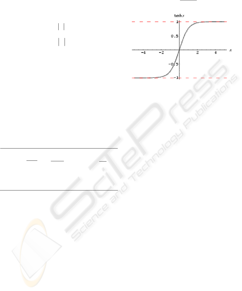
has the usual additional bias term. The activation
function used for the neurons of the hidden layer is
the hyperbolic tangent type (12, Fig. 5), while the
output layer nodes are linear. The four output
neurons have been exponentiated and normalized as
explained in section 2 to produce a probability
distribution. Control actions are selected at random
from this distribution.
sinh( )
tanh( )
cosh( )
z
z
z
=
(12)
Figure 5: The hyperbolic tangent function.
4 SIMULATED RESULTS
The controller was trained, as commmented in
section 3, in an episodic task. Robot and target
positions are reseted every 50 seconds so the total
amount of reward per episode percieved varies
depending on the episode. Even though the results
presented have been obtained as explained in section
3, in order to clarify the graphical results of time
convergence of the algorithm, for the plots below
some constrains have been applied to the simulator:
Target initial position is fixed to (0,0) and robot
initial location has been set to four random locations,
20x
=
±
and
20y
=
±
, therefore, the total amount
per episode when converged to minima will be the
same.
The number of episodes to be done has been set
to 100.000. For every episode, the total amount of
reward percieved is calculated. Figure 6 represents
the performance of the neural-network vehicle
controller as a function of the number of episodes,
when trained using OLPOMDP. The episodes have
been averaged over bins of 50 episodes. The
experiment has been repeated in 100 independent
runs, and the results presented are a mean over these
runs.
The simulated experiments have been repeated
and compared for different values of
α
and
β
.
1
K
g
−
·
·
N
s
K
gm
⎛⎞
⎜⎟
⎝⎠
2
2
·
·
Ns
K
gm
⎛⎞
⎜⎟
⎝⎠
N
K
g
⎛⎞
⎜⎟
⎝⎠
DIRECT GRADIENT-BASED REINFORCEMENT LEARNING FOR ROBOT BEHAVIOR LEARNING
229
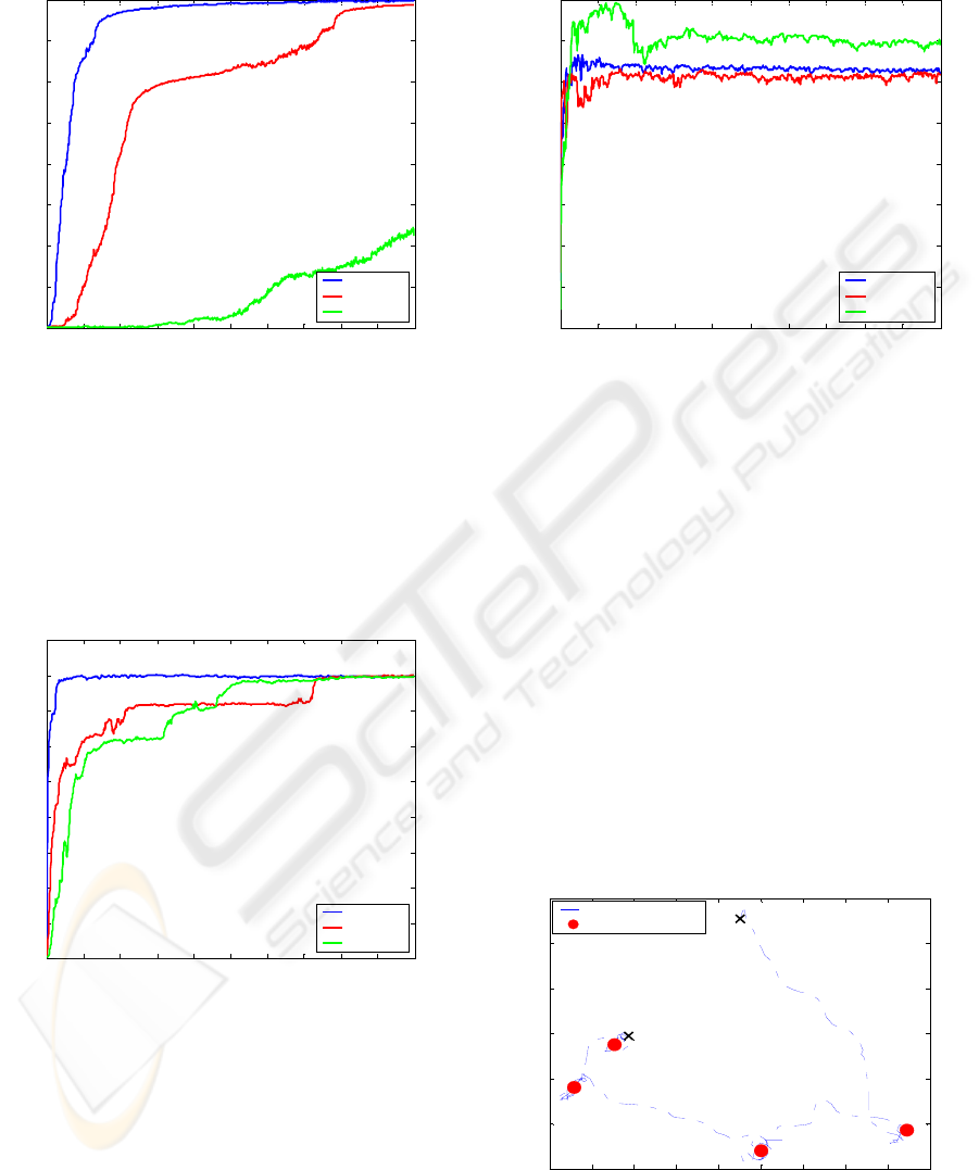
For
0.000001
α
=
:
0 200 400 600 800 1000 1200 1400 1600 1800 2000
-500
-450
-400
-350
-300
-250
-200
-150
-100
Total R per Episode, Averaged over bins of 50 Episodes (Alfa 0.000001)
Groups of 50 Episodes
Mean Total R per Episode
beta 0.999
beta 0.99
beta 0.97
Figure 6: Performance of the neural-network puck
controller as a function of the number of episodes.
Performance estimates were generated by simulating
100.000 episodes, and averaging them over bins of 50
episodes. Process repeated in 100 independent runs. The
results are a mean of these runs. Fixed
0.000001
α
=
, for
different values of
0.999
β
=
,
0.99
β
=
and
0.97
β
=
.
For
0.00001
α
=
:
0 200 400 600 800 1000 1200 1400 1600 1800 2000
-500
-450
-400
-350
-300
-250
-200
-150
-100
-50
Total R per Episode, Averaged over bins of 50 Episodes (Alfa 0.00001)
Groups of 50 Episodes
Mean Total R per Episode
beta 0.999
beta 0.99
beta 0.97
Figure 7: Performance of the neural-network puck
controller as a function of the number of episodes.
Performance estimates were generatedby simulating
100.000 episodes, and averaging them over bins of 50
episodes. Process repeated in 100 independent runs. The
results are a mean of these runs. Fixed
0.00001
α
=
, for
different values of
0.999
β
=
,
0.99
β
=
and
0.97
β
=
.
For
0.0001
α
=
:
0 200 400 600 800 1000 1200 1400 1600 1800 2000
-500
-450
-400
-350
-300
-250
-200
-150
-100
Total R per Episode, Averaged over bins of 50 Episodes (alfa 0.0001)
Groups of 50 Episodes
Mean Total R per Episode
beta 0.999
beta 0.99
beta 0.97
Figure 8: Performance of the neural-network puck
controller as a function of the number of episodes.
Performance estimates were generatedby simulating
100.000 episodes, and averaging them over bins of 50
episodes. Process repeated in 100 independent runs. The
results are a mean of these runs. Fixed
0.0001
α
=
, for
different values of
0.999
β
=
,
0.99
β
=
and
0.97
β
=
.
As it can bee apreciated in the figure above
(see Fig. 7), the optimal performance (within the
neural network controller used here) is around -100
for this simulated problem, due to the fact that the
puck and target locations are reset every 50 seconds
and for this reason the vehicle must be away from
target a fraction of the time. The best results are
obtained when
0.00001
α
=
and
0.999
β
=
, see Fig. 7.
Figure 9 represents the behavior of the trained
robot controller. For the purpose of the illustration,
only target location has been reseted to random
location, not the robot location.
-100 -80 -60 -40 -20 0 20 40 60 80
-100
-80
-60
-40
-20
0
20
INITIAL URIS POSITION
FINAL URIS POSITION
Target Following Task,Results After Learning
X Location
Y Location
URIS Trajectory
Target Positions
1
2
3
4
Figure 9: Behavior of a trained robot controller, results of
target following task asfter learning period is completed.
ICINCO 2005 - ROBOTICS AND AUTOMATION
230

5 CONCLUSIONS
An on-line direct policy search algorithm for AUV
control based on Baxter and Bartlett’s direct-gradient
algorithm OLPOMDP has been proposed. The method
has been applied to a real learning control system in
which a simulated model of the AUV URIS navigates a
two-dimensional world in a target following task. The
policy is represented by a neural network whose input is
a representation of the state, whose output is action
selection probabilities, and whose weights are the policy
parameters. The objective of the agent was to compute a
stochastic policy, which assigns a probability over each
of the four possible control actions.
Results obtained confirm some of the ideas
presented in section 1. The algorithm is easier to
implement compared with other RL methodologies like
value function algorithms and it represents a
considerable reduction of the computational time of the
algorithm. On the other side, simulated results show a
poor speed of convergence towards minimal solution.
In order to validate the performance of the
method proposed, future experiments are centered
on obtaining empirical results: the algorithm must be
tested on real URIS in a real environment. Previous
investigations carried on in our laboratory with RL
value functions methods with the same prototype
URIS (Carreras et al., 2003) will allow us to
compare both results. At the same time, the work is
focused in the development of a methodology to
decrease the convergence time of the RLDPS
algorithm.
ACKNOWLEDGMENTS
This research was esponsored by the spanish
commission MCYT (DPI2001-2311-C03-01). I
would like to give my special thanks to Mr. Douglas
Alexander Aberdeen of the Australian National
University for his help.
REFERENCES
R. Sutton and A. Barto, Reinforcement Learning, an
Introduction. MIT Press, 1998.
W.D. Smart and L.P Kaelbling, “Practical reinforcement
learning in continuous spaces”, International
Conference on Machine Learning, 2000.
N. Hernandez and S. Mahadevan, “Hierarchical memory-
based reinforcement learning”, Fifteenth International
Conference on Neural Information Processing
Systems, Denver, USA, 2000.
D.P. Bertsekas and J.N. Tsitsiklis, Neuro-Dynamic
Programming. Athena Scientific, 1996.
R. Sutton, D. McAllester, S. Singh and Y. Mansour,
“Policy gradient methods for reinforcement learning
with function approximation” in Advances in Neural
Information Processing Systems 12, pp. 1057-1063,
MIT Press, 2000.
C. Anderson, “Approximating a policy can be easier than
approximating a value function” Computer Science
Technical Report, CS-00-101, February 10, 2000.
R. Williams, “Simple statistical gradient-following
algorithms for connectionist reinforcement learning”
in Machine Learning, 8, pp. 229-256, 1992.
J. Baxter and P.L. Bartlett, “Direct gradient-based
reinforcement learning” IEEE International
Symposium on Circuits and Systems, May 28-31,
Geneva, Switzerland, 2000.
V.R. Konda and J.N. Tsitsiklis, “On actor-critic
algorithms”, in SIAM Journal on Control and
Optimization, vol. 42, No. 4, pp. 1143-1166, 2003.
S.P. Singh, T. Jaakkola and M.I. Jordan, “Learning
without state-estimation in partially observable
Markovian decision processes”, in Proceedings of the
11
th
International Conference on Machine Learning,
pp. 284-292, 1994.
N. Meuleau, L. Peshkin and K. Kim, “Exploration in
gradient-based reinforcement learning”, Technical
report AI Memo 2001-003, April 3, 2001.
J. Baxter and P.L. Bartlett, “Direct gradient-based
reinforcement learning I: Gradient estimation algorithms”
Technical Report. Australian National University, 1999.
P. Ridao, A. Tiano, A. El-Fakdi, M. Carreras and A.
Zirilli, “On the identification of non-linear models of
unmanned underwater vehicles” in Control
Engineering Practice, vol. 12, pp. 1483-1499, 2004.
D. A., Aberdeen, Policy Gradient Algorithms for Partially
Observable Markov Decision Processes, PhD Thesis,
Australian National University, 2003.
S. Haykin, Neural Networks, a comprehensive foundation,
Prentice Hall, Upper Saddle River, New Jersey, USA,
1999.
T.I., Fossen, Guidance and Control of Ocean Vehicles,
John Wiley and Sons, New York, USA, 1994.
J. A. Bagnell and J. G. Schneider, “Autonomous
Helicopter Control using Reinforcement Learning
Policy Search Methods”, in Proceedings of the IEEE
International Conference on Robotics and Automation
(ICRA), Seoul, Korea, 2001.
M. T. Rosenstein and A. G. Barto, “Robot Weightlifting
by Direct Policy Search”, in Proceedings of the
International Joint Conference on Artificial
Intelligence, 2001.
N. Kohl and P. Stone, “Policy Gradient Reinforcement
Learning for Fast Quadrupedal Locomotion”, in
Proceedings of the IEEE International Conference on
Robotics and Automation (ICRA), 2004.
M. Carreras, P. Ridao and A. El-Fakdi, “Semi-Online
Neural-Q-Learning for Real-Time Robot Learning”, in
Proceedings of the IEEE/RSJ International
Conference on Intelligent Robots and Systems (IROS),
Las Vegas, USA, 2003.
DIRECT GRADIENT-BASED REINFORCEMENT LEARNING FOR ROBOT BEHAVIOR LEARNING
231
