
CONTROL OF AN ASYMMETRICAL OMNI DIRECTIONAL
MOBILE ROBOT
Seyed Mohsen Safavi, Mohammad Ajoodanian, Ahmad movahedian
Mechanical Engineering Department, Isfahan University Of Technologhy (IUT) ,Isfahan,Iran
Keywords: Holonomic Omnidirectional mobile robot; Asymmetrical Structure.
Abstract: This paper describes how to control an asymmetric wheeled mobile robot with omnidirectional wheels,
considering the sample of a robot with three wheels. When flexible motion capabilities are required this
robot must be designed to meet the related requirements, namely fast and agile motions as well as robust
navigation. This paper provides an overview for the design of kinematics and dynamics of the robot, as well
as the motion and velocities equations. In addition to the above, a control method to obtain a proper control
model is explained. Simulation example is presented to demonstrate the ability of this control method. The
implementation and test of the controller on the real robot gives the results compatible with the simulation.
It was learned that the discontinuities between omnidirectional wheels’ rollers play an important role in
decreasing the accuracy of motion.
1 INTRODUCTION
Omnidirectional vehicles provide superior
maneuvering capability compared to the more
common car-like vehicles. The ability to move along
any direction, irrespective of the orientation of the
vehicle, makes it an attractive option in dynamic
environments. The annual RoboCup competition,
where teams of fully autonomous robots engage in
soccer matches, is an example of where
omnidirectional vehicles have been used in
computationally intensive dynamic environments
(Kalmár-Nagy et al., 2004) (Veloso et al., 1999)
(Kitano et al., 1998).
Among omnidirectional mobile robots, the one with
three or more wheels is more powerful. A holonomic
system is one in which the number of degrees of
freedom (DOF) is equal to the number of
coordinates needed to specify the configuration of
the system. In the field of mobile robots, the term
holonomic mobile robot is applied to the abstraction
called the robot, or base, without regard to the rigid
bodies which make up the actual mechanism. Thus,
any mobile robot with three degrees of freedom of
motion in the plane has become known as a
holonomic mobile robot (Holmberg et al., 1999).
Many different control mechanisms have been
created to achieve holonomic motion (Jung et al,.
1999) (Moore er al., 1999). In addition, these
systems have symmetric mechanisms. The
symmetric mobile robots with 3 DOF mostly have
120-degree angles between the wheels and the full
structure includes 3 actuators as well as 3 wheels
(Kalmár-Nagy et al., 2004). The control procedure
of such robots has been the subject of discussion in
several research papers. However in small robots (18
cm diameter of base) there is not enough space to
accommodate other components and the change in
angles between the wheels would partially overcome
this problem. The angle between front wheels is
140˚ and the two other angles are 110˚, which causes
asymmetric problem in robot and its control system.
The objective of this paper is to establish a real time
control strategy that could move the asymmetrical
robot to a given location with zero final velocity as
quickly as possible based on measurement of the
vehicle position and orientation.
The paper is ordered in such a way to describe the
Persia Robot system followed by the kinematics and
dynamic model of asymmetric omnidirectional robot
vehicle. Then Simulations and PD control method
are presented. The paper ends with the concluding
remarks.
120
Mohsen Safavi S., Ajoodanian M. and movahedian A. (2005).
CONTROL OF AN ASYMMETRICAL OMNI DIRECTIONAL MOBILE ROBOT.
In Proceedings of the Second International Conference on Informatics in Control, Automation and Robotics - Robotics and Automation, pages 120-125
DOI: 10.5220/0001188501200125
Copyright
c
SciTePress
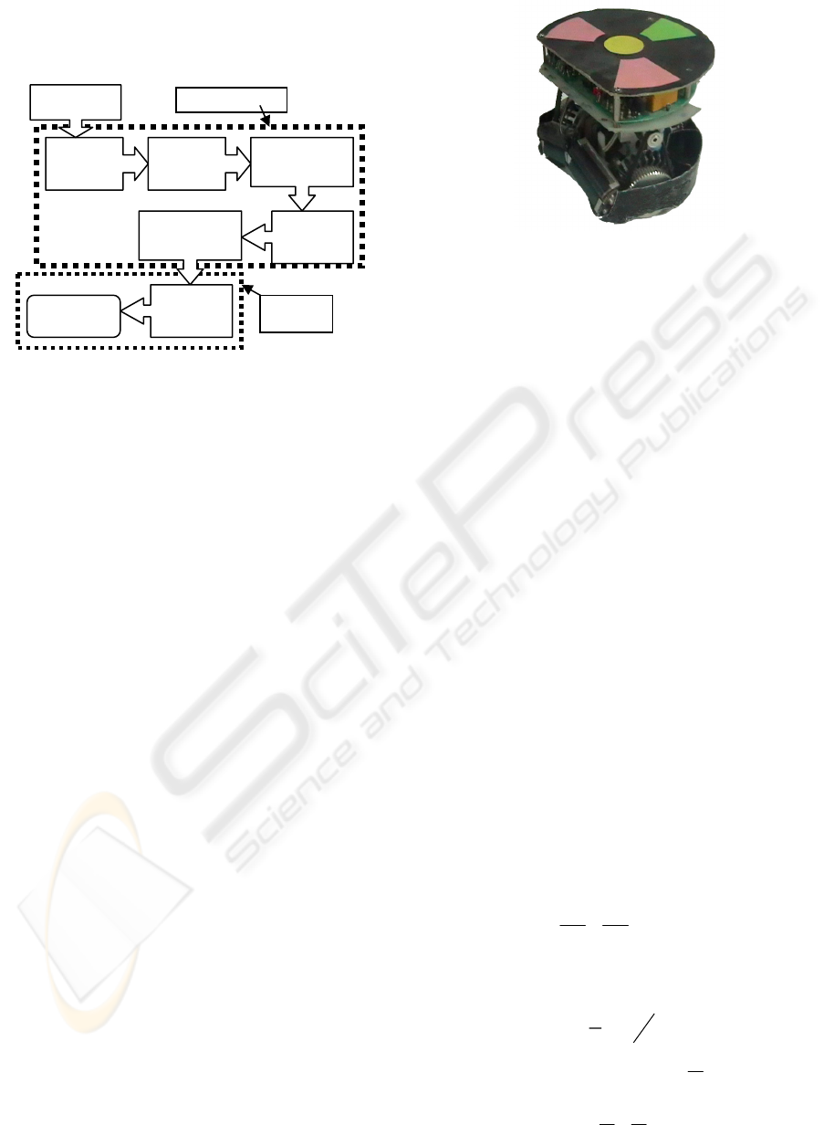
2 ROBOPERSIA SYSTEM
OVERVIEW
The complete RoboPersia system is a layered set of
subsystems which is shown in Figure 1. Figure 2
shows a photograph of the RoboPersia. An overhead
camera captures global images of the field. The
vision software processes the images to identify the
location and the velocity of robots and the ball. This
state of the field is passed to the Decision-Making
System (DMS). DMS is the highest level planner in
the system, responsible for distributing the overall
goal of the team amongst the individual robots.
DMS is responsible for the multi-robot coordination
and cooperation by selecting a role for each robot.
Some example roles include ATTACK and
DEFEND. The DMS roles and role parameters with
the field state are sent to the Role Layer which is
responsible for executing roles by selecting
behaviour for each robot. Some example behaviours
include KICK and MOVE. Behaviours and
behaviour parameters with the field state are passed
to Behaviour Layer. The Behaviour Layer attempts
to execute the desired behaviour by dedicating the
proper motion while avoiding obstacles. This layer
determines the immediate desired heading and
distance for the control layer .The Control Layer,
based on PD controller, controls the position and
head of the robots by changing the actuators duty
cycles. The feedback comes from the state of the
field
.
2.1 Optimizing the Omni Directional
Wheel
The holonomic and non-holonomic omnidirectional
mobile robot has been studied by using a variety of
mechanism. Several omnidirectional platforms have
been known to be realized by developing a
specialized wheel or mobile mechanisms (Holmberg
et al., 1999). These include various arrangements of
universal or omni wheels (La 1979; Carlisle 1983),
double universal wheels (Bradbury 1977), Swedish
or Mecanum wheels (Ilon 1971), chains of spherical
wheels (West and Asada 1992) or cylindrical wheels
(Hirose and Amano 1993), orthogonal wheels
(Killough and Pin 1992), ball wheels (West and
Asada 1994) and omni directional poly roller wheel
(Asama, 1995, Watanaba, 1998). All of these
mechanisms, except for some types with ball wheels,
have discontinuous wheel contact points which are a
great source of vibration; primarily because of the
changing support provided; and often additionally
because of the discontinuous changes in wheel
velocity needed to maintain smooth base motion
(Watanabe, 1998) (Williams et al., 2002) (Pin et al.,
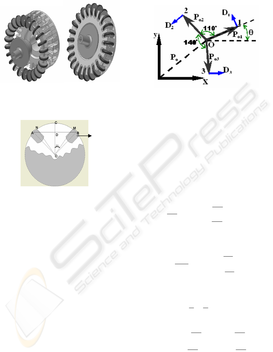
1994) (Diegel et al., 2002). In order to decrease the
vibration of the platform, the number of little rollers
was increased from 12 per wheel, which was used in
the previous design to 22 with the constant diameter
(Fig. 3). The run-out is decreased nearly 0.08-
0.1mm.It’s where the previous run out was 1mm. An
equation was derived for determining the run out,
namely to find how much a given wheel design will
bounce up and down as it rotates (run-out). The
derivation is relatively straightforward procedure by
using trigonometry, and the resulting formula is
shown below in which n is the number of the rollers
and R is radius of the wheel (Fig. 4).
(1)
BOMBOCo
∠
−
∠
=
∠
1 (2)
(3)
(4)
(5)
Figure 2: RoboPersia
Figure 1: Complete RoboPersia System
Global
Vision
Decision
Making
Role Laye
r
Behavior
Layer
Control
Layer
Onboard
Controller
Actuato
r
Robo
t
Off Field PC
Camera
)1cos1( oRODOCoutRun
Max
−=−=−
)
2
(*
2
1
n
BOC
π
=∠
R
BOMBOMR
2
2* =∠⇒=∠
)
2
(1
Rn
O −=∠∴
π
CONTROL OF AN ASYMMETRICAL OMNI DIRECTIONAL MOBILE ROBOT
121
⎥
⎦
⎤
⎢
⎣
⎡
=
0
1
1
L
o
P
3 ROBOT KINEMATIC
Omni directional robots usually use special wheels,
which were described in the preceding section. The
body of each wheel is connected to the DC motor
shaft. Therefore, a robot with three omni directional
wheels can equilibrate on plane easily and follow
any trajectory. Our robot structure includes three
special omni-directional wheels for the motion
system as shown in Fig.3.
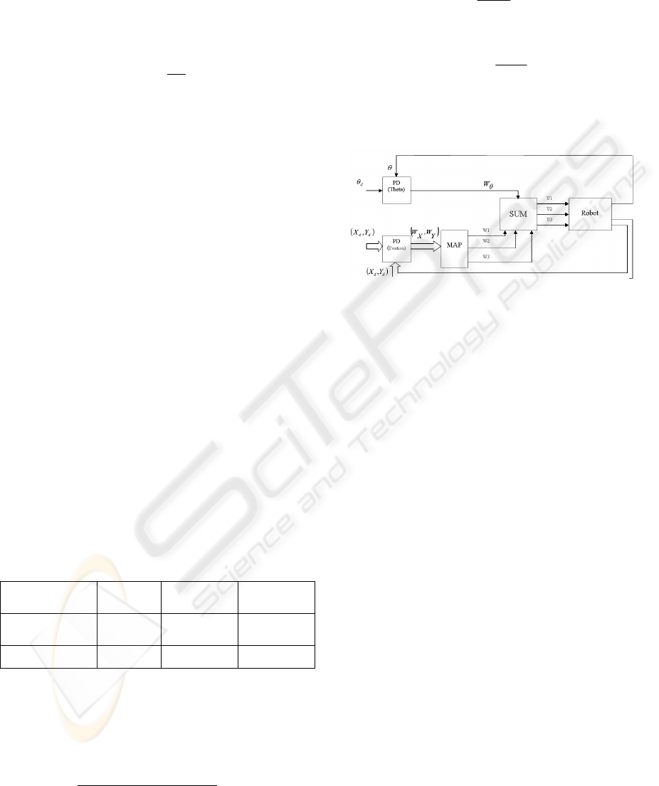
3.1 Kinematics Modeling
Using omni directional wheels, the schematic view
of robot kinematics can be shown in Fig. 5 (Kalmar-
Nagy, T., 1998), where O is the robot center of
mass, Po is defined as the vector connecting O to the
origin and D is the drive direction vector of each
wheel and θ is the angle of counter clockwise
rotation. Unitary rotation matrix, [R (
θ
)] is defined
as:
(6)
The position vectors {P
o1
},…,{P
o3
}with respect to
the local coordinates centered at the robot center of
mass are given as:
(7)
(8)
(9)
Where, L is the distance of wheels from the robot
canter of mass (O).
(10)
(11)
Figure 3: The explosive view of new omni
directional wheel and Omni directional Wheel
()
[]
⎟
⎟
⎠
⎞
−
⎜
⎜
⎝
⎛
=
θ
θ
θ
θ
θ
cos
sin
sin
cos
R
°
=
∠
110,
21 oo
PP
⎥
⎥
⎥
⎦
⎤
⎢
⎢
⎢
⎣
⎡
=
⎟
⎠
⎞
⎜
⎝
⎛
=
)
18
11
sin(
)
18
11
cos(
18
π11
1o2
π
π
L
o
PRP
°
−
=
∠
110,
31 oo
PP
⎥
⎥
⎥
⎥
⎦
⎤
⎢
⎢
⎢
⎢
⎣
⎡
⎟
⎠
⎞
⎜
⎝
⎛
−
⎟
⎠
⎞
⎜
⎝
⎛
=
⎟
⎠
⎞
⎜
⎝
⎛
−
=
18
11
18
11
18
11
1o3
π
π
π
Sin
Cos
L
o
PRP
oii
L
PRD
⎟
⎠
⎞
⎜
⎝
⎛
=
2
1
π
⎥
⎥
⎥
⎥
⎦
⎤
⎢
⎢
⎢
⎢
⎣
⎡
=
⎥
⎥
⎥
⎥
⎦
⎤
⎢
⎢
⎢
⎢
⎣
⎡
−
=
⎥
⎦
⎤
⎢
⎣
⎡
=
)
18
11
cos(
)
18
11
sin(
,
)
18
11
cos(
)
18
11
sin(
,
1
0
321
π
π
π
π
DDD
Rolle
Figure 4: Schematic of Omni directional.
Figure 5: Omnidirectional Robot Model, Top View.
ICINCO 2005 - ROBOTICS AND AUTOMATION
122

T
L
L
L
⎟
⎟
⎟
⎟
⎟
⎟
⎠
⎞
⎜
⎜
⎜
⎜
⎜
⎜
⎝
⎛
+−+
−−−−
−
=
∧
)
18
7
cos()
18
7
sin(
)
18
7
cos()
18
7
sin(
cossin
)(
θ
π
θ
π
θ
π
θ
π
θθ
θ
P
3.2 Equation of motion and
velocities
Using the above notations, the wheel position and
velocity vectors can be expressed using rotation
matrix [R (
θ
)] as:
0
()
ioi
θ
=+rPR P
(12)
0
()
ioi
θ
•
=+vPRP
(13)
The vector P
o
=(x y)
T
is the position of the center of
mass with respect to Cartesian coordinates. The
individual wheel velocities are
(14)
Substituting equation (13) into equation (14) results
in:
(15)
Note that the second term in the right hand side is
the tangential velocity of the wheel. This tangential
velocity could be also written as:
(16)
From the kinematics model of the robot, it is clear
that the wheel velocity is a function of linear and
angular velocities of robot center of mass, i.e.:
(17)
4 DYNAMIC EQUATIONS
Linear and angular momentum balance can be
written as;
(18)
(19)
Where
i
f is the magnitude of the force produced by
the ith motor, m is the mass of the robot and J is its
moment of inertia.
f =αU −βv (20)
Where
f is the magnitude of the force generated by
a wheel attached to the motor, and v (m/s) is the
velocity of the wheel. The constants α (N/V) and β
(kg/s) can readily be determined from experiment or
from motor catalogue.
Substituting equation (20) into equation (18) and
(19) yields:
(21)
(22)
This system of differential equations can be written
in the following form (Kalmár-Nagy et al., 2004):
(23)
With
(24)
And
(25)
So that the non-dimensional equations of motion
become(Kalmár-Nagy et al., 2004):
(26)
Where q(θ, t) is the control action(Kalmár-Nagy et
al., 2004):
q(θ, t) = P(θ)U(t) (27)
()
)]([
i
T
ii
DRv
θυ
=
i
T
T
oii
T
o
i
DRRPDRP
.
)()()(
θθθυ
⋅
+=
i
T
T
oi
L DRRP )()(
θθθ
⋅⋅
=
⎟
⎟
⎟
⎟
⎟
⎟
⎠
⎞
⎜
⎜
⎜
⎜
⎜
⎜
⎝
⎛
⎟
⎟
⎟
⎟
⎟
⎟
⎠
⎞
⎜
⎜
⎜
⎜
⎜
⎜
⎝
⎛
+−+
−−−−
−
=
⎟
⎟
⎟
⎠
⎞
⎜
⎜
⎜
⎝
⎛
⋅
⋅
⋅
θ
θ
π
θ
π
θ
π
θ
π
θθ
y
x
L
L
L
v
v
v
)
18
7
cos()
18
7
sin(
)
18
7
cos()
18
7
sin(
cossin
3
2
1
⋅⋅
=
=
∑
0
3
1
)( PDR mf
i
ii
θ
∑
=
⋅⋅
=
3
1i
i
JfL
θ
∑
=
=−
3
1
..
0
)()(
i
iii
mvU PDR
θβα
∑
=
=−
3
1
..
)(
i
ii
JvUL
θβα
⎟
⎟
⎟
⎟
⎟
⎟
⎟
⎠
⎞
⎜
⎜
⎜
⎜
⎜
⎜
⎜
⎝
⎛
−=
⎟
⎟
⎟
⎟
⎟
⎟
⎠
⎞
⎜
⎜
⎜
⎜
⎜
⎜
⎝
⎛
∧
.
2
.
.
..
..
..
2
2
3
)()(
θ
β
θα
θ
L
y
x
t
J
ym
xm
UP
⎟
⎟
⎟
⎠
⎞
⎜
⎜
⎜
⎝
⎛
=
)(
)(
)(
)(
3
2
1
tU
tU
tU
tU
),(
2
.
2
.
.
..
..
..
t
J
mL
y
x
y
x
θ
θθ
q=
⎟
⎟
⎟
⎟
⎟
⎟
⎟
⎠
⎞
⎜
⎜
⎜
⎜
⎜
⎜
⎜
⎝
⎛
+
⎟
⎟
⎟
⎟
⎟
⎟
⎠
⎞
⎜
⎜
⎜
⎜
⎜
⎜
⎝
⎛
CONTROL OF AN ASYMMETRICAL OMNI DIRECTIONAL MOBILE ROBOT
123
5 POSITION CONTROL AND
IMPLEMENTATION
In order to control the position and head angle of
robot a PD controller is employed. Mathematically a
PD controller can be expressed as
(28)
By increasing K
p
the rise time becomes faster, but on
the other hand the overshoot increases too, which is
undesired. Furthermore the stability gets worse.
Derivative control improves system performance in
two ways. Firstly, it adds positive phase angles to
increase the open-loop frequency response so as to
improve system stability and to increase close-loop
system bandwidth to increase the speed of response.
Secondly, it provides braking when the response is
getting closing to the new set point. This braking
action not only helps to reduce overshoot but also
tends to reduce steady-state error. Influence of
derivative control on the system is proportional to
K
d
, but increasing derivative feedback will slow the
system response and magnify any noise that may be
present. It is important to note that derivative control
has no influence on the accuracy of the system, but
just on the response time.
A problem that can occur with derivative control is
that in a real control system, the set point is usually
stepped up or down in discrete steps. A step change
has an infinitely positive slope, which will saturate
the derivative function. A solution to this problem is
to base the derivative control on the feedback signal
alone instead of the error because the controlled
variable can never actually change instantaneously,
even if the set point does. The effect of proportional
and derivative action is summarized in table 1.
Table 1: Controller properties
Action Rise
Time
Overshoot Stability
Increasing K
p
Faster Increases Gets
worse
Increasing K
d
Slower Decreases Improves
A digital controller is used for our purpose. For
digital filter differentiation of a function e(t) the
following technique is used. The slope of e (t) at the
t = kT is approximated to be slope of the straight line
connecting e[(k-1)T] with e(kT). Numerical
derivative of e (t) at t=kT can be written as
(29)
The z-transform of this equation yields
(30)
So the digital PD controller can be written as
(31)
We use this equation to implement the controller. As
depicted in Fig.6, the position and the angle of the
robot is obtained by using a camera.
These measurements are compared with the desired
set-point values and the calculated errors. The
camera also gives the derivative of output values.
The error in position is fed to a digital PD (position
PD). Position PD output is applied to a limiter and
then mapped to direction of each wheel by an
appropriate function block (W1, W2, W3). Error in
robot angle is fed to another PD (head angle
PD).Head angle PD output (W
θ
) is limited and then
added to the outputs of mapping block.
(32)
These signals determine the duty cycle of each robot
motor.
To tune the PDs, the following procedure is pursued.
The derivative action removed by setting K
d
=0, the
gain K
p
is tuned to give the desired response and K
d
is adjusted to damp the overshoot. The above steps
are repeated until an acceptable response is
achieved.
To demonstrate the computational efficiency and
robustness of the algorithm, simulations were
performed (with m=3kg, j=0.014 Kgm
2
, L=0.07m).
Position and velocity of the vehicle are assumed to
be measured 50 times per second. The inputs to the
algorithm are initial and desired positions and head
angle.
dt
de
TeKK
dp
+=
z
z
zD
1
)(
−
=
⎥
⎦
⎤
⎢
⎣
⎡
−
+=
z
z
KKK
dp
1
⎪
⎩
⎪
⎨
⎧
+=
+=
+=
θ
θ
θ
WWU
WWU
WWU
33
22
11
T
TkekTe
D
])1[()( −−
=
Figure 6: Control Diagram
ICINCO 2005 - ROBOTICS AND AUTOMATION
124
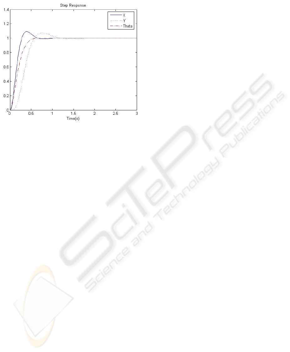
The results are shown in Fig. 7.As depicted, the
robots head angle overshoot is smaller than X
overshoot and y overshoot.
6 CONCLUSIONS
Wheeled mobile robots (WMRs) are increasingly
present in industrial and service robotics,
particularly when flexible motion capabilities are
required on reasonably smooth ground and surface
(Schraft et al., 1998). Several mobility
configurations (wheel number and type, their
location and actuation, single or multi-body
structure) can be found in the applications (Jones et
al., 1993), which can be lead to designing and
implementing an asymmetric robot.
This paper has presented a control model for a
specific kind of asymmetric omnidirectional
wheeled mobile robot. During initial modelling and
experimental works, it was supposed that
asymmetric feature could be a limitation for robot to
meet the requirements. While this is true, it was
however learned that if we derive proper control
model for robot we can overcome this limitation to
some extent. Since our objective was to model the
control of a specific kind of an asymmetric
omnidirectional wheeled mobile robot, this paper did
not develop a method for a large variety of
asymmetric robots. A control method that depends
on the angles between robot wheels, and includes
motion and velocity equations are supposed to be
developed in the future studies as extension of this
work.
REFERENCES
Tamás Kalmár-Nagy, Raffaello D’Andrea ,Pritam
Ganguly 2004. “Near-optimal dynamic trajectory
generation and control of an omnidirectional vehicle”.
Robotics and Autonomous Systems 46 (2004) 47–64
M. Veloso, E. Pagello, H. Kitano (Eds.), RoboCup-99:
Robot Soccer World Cup III, Lecture Notes in
Computer Science, 1856 Springer,New York, 2000
H. Kitano, J. Siekmann, J.G. Garbonell (Eds.), RoboCup-
97: Robot Soccer World Cup I, Vol. 139, Lecture
Notes in Computer Science 1395, Springer, New
York, 1998.
Robert Holmberg_ and Oussama Khatib,” Development of
a Holonomic Mobile Robot for Mobile Manipulation
Tasks”. FSR’99 International Conference on Field and
Service Robotics, Pittsburgh, PA, Aug. 1999
M. Jung, H. Shim, H. Kim, J. Kim, The miniature omni-
directional mobile robot OmniKity-I (OK-I),
Proceedings of the InternationalConference on
Robotics and Automation 4 (1999) 2686–2691.
K.L. Moore, N.S. Flann, Hierarchial task decomposition
approach to path planning and control for an omni-
directional autonomous mobile robot, Proceedings of
the International Symposium on Intelligent
Control/Intelligent Systems and Semiotics (1999)
302–307.
Keigo Watanabe, 1998,"Control of an Omnidirectional
Mobile Robot", 1998 Second International Conference
on Knowledge Based Intelligent Electronic System,
Adelaide Australia
Robert L. Williams, II, Member, IEEE, Brian E. Carter,
Paolo Gallina, and Giulio Rosati. Dynamic Model
With Slip for Wheeled Omnidirectional Robots. IEEE
Transactions On Robotics and Automation, VOL. 18,
NO. 3, JUNE 2002.
Francois G. Pin, Stephan M.Killough,1994."A New
Family of Omnidirectional and Holonomic Wheeled
Platforms for Mobile Robots," IEEE Trans. On
Robotics and Automation, vol 10,no.4,pp.480-
489,1994
Olaf Diegel, Aparna Badve, Glen Bright, Johan Potgieter,
Sylvester Tlale,"Improved Mecanum Wheel Design
for Omni-directional Robots",Proc. 2002 Australasian
Conference on Robotics and Automation Auckland,
November 2002.
Schraft R D, Schmierer G 1998 Serviceroboter . Springer,
Berlin
Jones J L, Flynn A M 1993 Mobile Robots: Inspiration to
Implementation. A K Petters,Wellesly, MA
)1,1,1,0
0
,0
0
,0
0
( rad
d
m
d
Ym
d
XYX ==
=
===
θ
θ
Figure 7: Step Response
CONTROL OF AN ASYMMETRICAL OMNI DIRECTIONAL MOBILE ROBOT
125
