
KINEMATIC AND SINGULARITY ANALYSIS OF THE
HYDRAULIC SHOULDER
A 3-DOF Redundant Parallel Manipulator
H. Sadjadian and H. D. Taghirad
Advanced Robotics and Automated Systems (ARAS),
Electrical Engineering Department,
K.N. Toosi University of Technology
P.O. Box 16315-1355, Tehran, Iran
Keywords: Parallel Manipulator, Kinematic Modeling, Forward Kinematics, Jacobian, Singularity Analysis.
Abstract: In this paper, kinematic modeling and singularity analysis of a three DOF redundant parallel manipulator
has been elaborated in detail. It is known, that on the contrary to series manipulators, the forward kinematic
map of parallel manipulators involves highly coupled nonlinear equations, whose closed-form solution
derivation is a real challenge. This issue is of great importance noting that the forward kinematics solution is
a key element in closed loop position control of parallel manipulators. Using the novel idea of kinematic
chains recently developed for parallel manipulators, both inverse and forward kinematics of our parallel
manipulator are fully developed, and a closed-form solution for the forward kinematic map of the parallel
manipulator is derived. The closed form solution is also obtained in detail for the Jacobian of the
mechanism and singularity analysis of the manipulator is performed based on the computed Jacobian.
1 INTRODUCTION
Over the last two decades, parallel manipulators
have been among the most considerable research
topics in the field of robotics. A parallel manipulator
typically consists of a moving platform that is
connected to a fixed base by several legs. The
number of legs is at least equal to the number of
degrees of freedom (DOF) of the moving platform
so that each leg is driven by no more than one
actuator, and all actuators can be mounted on or near
the fixed base. These robots are now used in real-life
applications such as force sensing robots, fine
positioning devices, and medical applications
(Merlet, 2002).
In the literature, mostly 6 DOF parallel mechanisms
based on the Stewart-Gough platform are analyzed
(Joshi et al., 2003). However, parallel manipulators
with 3 DOF have been also implemented for
applications where 6 DOF are not required, such as
high-speed machine tools. Recently, 3 DOF parallel
manipulators with more than three legs have been
investigated, in which the additional legs separate
the function of actuation from that of constraints at
the cost of increased mechanical complexity (Joshi
et al., 2003). Complete kinematic modeling and
Jacobian analysis of such mechanisms have not
received much attention so far and is still regarded
as an interesting problem in parallel robotics
research. It is known that unlike serial manipulators,
inverse position kinematics for parallel robots is
usually simple and straight-forward. In most cases
joint variables may be computed independently
using the given pose of the moving platform. The
solution to this problem is in most cases uniquely
determined. But forward kinematics of parallel
manipulators is generally very complicated. Its
solution usually involves systems of nonlinear
equations which are highly coupled and in general
have no closed form and unique solution. Different
approaches are provided in literature to solve this
problem either in general or in special cases. There
are also several cases in which the solution to this
problem is obtained for a special or novel
architecture (Baron et al., 2000, Merlet, 96, Song et
al., 2001, Bonev et al., 2001). Two such special 3
DOF constrained mechanisms have been studied in
(Siciliano, 99, Fattah et al., 2000), where kinematics,
Jacobian and dynamics have been considered for
125
Sadjadian H. and D. Taghirad H. (2005).
KINEMATIC AND SINGULARITY ANALYSIS OF THE HYDRAULIC SHOULDER - A 3-DOF Redundant Parallel Manipulator.
In Proceedings of the Second International Conference on Informatics in Control, Automation and Robotics - Robotics and Automation, pages 125-131
DOI: 10.5220/0001185301250131
Copyright
c
SciTePress

such manipulators. Joshi and Tsai (Joshi et al., 2003)
performed a detailed comparison between a 3-UPU
and the so called Tricept manipulator regarding the
kinematic, workspace and stiffness properties of the
mechanisms. In general, different solutions to the
forward kinematics problem of parallel manipulators
can be found using numerical or analytical
approaches, or closed form solution for special
architectures (Didrit et al., 98, Dasgupta et al.,
2000).
In this paper, complete kinematic modeling has been
performed and a closed-form forward kinematics
solution is obtained for a three DOF actuator
redundant hydraulic parallel manipulator. The
mechanism is designed by Hayward (Hayward, 94),
borrowing design ideas from biological manipulators
particularly the biological shoulder. The interesting
features of this mechanism and its similarity to
human shoulder have made its design unique, which
can serve as a basis for a good experimental setup
for parallel robot research.
In a former study by the authors, different numerical
approaches have been used to solve the forward
kinematic map of this manipulator (Sadjadian et al.,
2004). The numerical approaches are an alternative
to estimate the forward kinematic solution, in case
such solutions cannot be obtained in closed form. In
this paper, however, the novel idea of kinematic
chains developed for parallel manipulators structures
(Siciliano, 99, Fattah et al., 2000), is applied for our
manipulator, and it is observed that in a systematic
manner the closed form solution for this manipulator
can also be obtained in detail.
The paper is organized as following: Section 2
contains the mechanism description. Kinematic
modeling of the manipulator is discussed in section
3, where inverse and forward kinematics is studied
and the need for appropriate method to solve the
forward kinematics is justified. In section 4, The
Jacobian matrix of the manipulator is derived
through a complete velocity analysis of the
mechanism, and finally, in section 5, singularity
analysis is performed using the configuration-
dependent Jacobian.
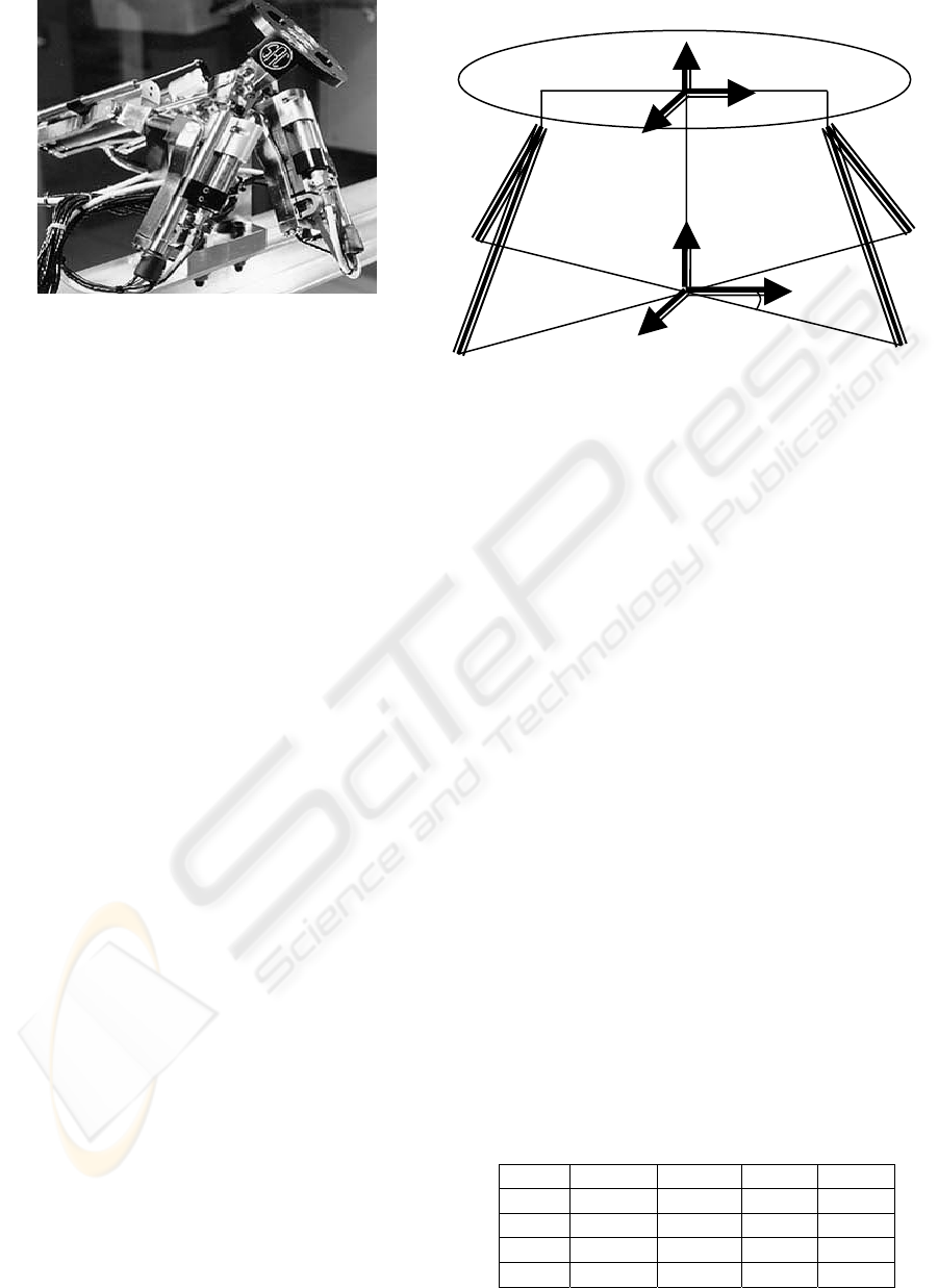
2 MECHANISM ESCRIPTION
A schematic of the mechanism, which is currently
under experimental studies in ARAS Robotics Lab,
is shown in Fig. 1. The mobile platform is
constrained to spherical motions. Four high
performance hydraulic piston actuators are used to
give three degrees of freedom in the mobile
platform. Each actuator includes a position sensor of
LVDT type and an embedded Hall Effect force
sensor. The four limbs share an identical kinematic
structure. A passive leg connects the fixed base to
the moving platform by a spherical joint, which
suppresses the pure translations of the moving
platform. Simple elements like spherical and
universal joints are used in the structure. A complete
analysis of such a careful design will provide us with
required characteristics regarding the structure itself,
its performance, and the control algorithms.
From the structural point of view, the shoulder
mechanism which, from now on, we call it "the
Hydraulic Shoulder" falls into an important class of
robotic mechanisms called parallel robots. In these
robots, the end effector is connected to the base
through several closed kinematic chains. The
motivation behind using these types of robot
manipulators was to compensate for the
shortcomings of the conventional serial manipulators
such as low precision, stiffness and load carrying
capability. However, they have their own
disadvantages, which are mainly smaller workspace
and many singular configurations. The hydraulic
shoulder, having a parallel structure, has the general
features of these structures. It can be considered as a
shoulder for a light weighed seven DOF robotic arm,
which can carry loads several times, its own weight.
Simple elements, used in this design, add to its
lightness and simplicity. The workspace of such a
mechanism can be considered as part of a spherical
surface. The orientation angles are limited to vary
between -π/6 and π/6. No sensors are available for
measuring the orientation angles of the moving
platform which justifies the importance of the
forward kinematic map as a key element in feedback
position control of the shoulder with the LVDT
position sensors used as the output of such a control
scheme.
3 KINEMATICS
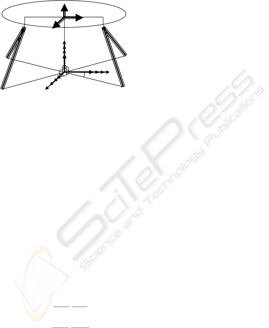
Fig. 2 depicts a geometric model for the hydraulic
shoulder manipulator which will be used for its
kinematics derivation.
The parameters used in kinematics can be defined
as:
ib
CAl = , CPl
p
=
4
y
id
PPl =
4
z
ik
PPl =
:α The angle between
4
CA and
0
y
:C Center of the reference frame
:P Center of the moving plate
:
i
l Actuator lengths i=1, 2, 3, 4
:
P
i
Moving endpoints of the actuators
:
A
i
Fixed endpoints of the actuators
ICINCO 2005 - ROBOTICS AND AUTOMATION
126
1
l
2
l
3
l
4
l
C
1
A
2
A
3
A
4
A
1
P
2
P
d
l
k
l
0
X
4
X
α
0
Y
4
Y
0
Z
4
Z
b
l
p
l
P
}{A
}{B
Figure 1: The hydraulic shoulder in movement
Two coordinate frames are defined for the purpose
of analysis. The base coordinate frame {A}:
000
zyx is
attached to the fixed base at point C (rotation center)
with its
0
z
-axis perpendicular to the plane defined
by the actuator base points
4321
AAAA and an
0
x -axis
parallel to the bisector of angle ∠A
1
CA
4
. The
second coordinate frame {B}:
444
zyx
is attached to
the center of the moving platform P with its z-axis
perpendicular to the line defined by the actuators
moving end points (P
1
P
2
) along the passive leg. Note
that we have assumed that the actuator fixed
endpoints lie on the same plane as the rotation center
C. The position of the moving platform center P is
defined by:
T
zyx
A
pppp ],,[=
(1)
Also, a rotation matrix
B
A
R is used to define the
orientation of the moving platform with respect to
the base frame:
)(θ)R(θ)R(θR
xxyyzz
=
B
A
R
⎥
⎥
⎥
⎦
⎤
⎢
⎢
⎢
⎣
⎡
−
−+
+−
=
xyxyy
xzxyzxzxyzyz
xzxyzxzxyzyz
ccscs
sccssccssscs
sscsccsssccc
θθθθθ
θθθθθθθθθθθθ
θθθθθθθθθθθθ
(2)
where
zyx
θ
θ
θ
,, are the orientation angles of the
moving platform denoting rotations of the moving
frame about the fixed
,, y
x
and
z
axes respectively.
Also
θ
c and
θ
s denote )cos(
θ
and )sin(
θ
respectively.
With the above definitions, the
44 × transformation
matrix
B
A
T is easily found to be:
⎥
⎦
⎤
⎢
⎣
⎡
=
10
pR
T
A
B
A
B
A
(3)
Hence, the position and orientation of the moving
platform are completely defined by six variables,
from which, only three orientation angles
zyx
θ
θ
θ
,, are
independently specified as the task space variables
of the hydraulic shoulder.
Figure 2: A geometric model for the hydraulic shoulder
manipulator
3.1 Inverse Kinematics
In modeling the inverse kinematics of the hydraulic
shoulder we must determine actuator lengths (
i
l ) as
the actuator space variables given the task space
variables
zyx
θ
θ
θ
,, as the orientation angles of the
moving platform. First, note that the passive leg
connecting the center of the rotation to the moving
platform can be viewed as a 3-DOF open-loop chain
by defining three joint variables
,,
21
θ
θ
and
3
θ
as the
joint space variables of the hydraulic shoulder.
Hence, applying the Denavit-Hartenberg (D-H)
convention, the transformation
B
A
T can also be
written as:
B
A
B
A
TTTTT
3
33
2
22
1
11
).().().(
θθθ
=
(4)
The D-H transformation matrices
j
i
T are computed
using the coordinate systems for the passive leg in
Fig. 3, according to the D-H convention. As shown
in Fig. 3, the
0
x axis of frame {A} points along the
first joint axis of the passive leg; the first link frame
is attached to the first moving link with its
1
x axis
pointing along the second joint axis of the passive
leg; the second link frame is attached to the second
moving link with its
2
x axis pointing along the third
joint axis of the passive leg; and the third link frame
is attached to the moving platform in accordance
with the D-H convention. Using the above frames,
the D-H parameters of the passive leg are found as
in Table (1).
Table 1: D-H Parameters for the passive supporting leg
i
1−i
α
1−i
a
i
d
i
θ
1
°
90 0 0
1
θ
2
°
90
0 0
2
θ
3
°
90 0 0
3
θ
B 0 0
p
l 0
KINEMATIC AND SINGULARITY ANALYSIS OF THE HYDRAULIC SHOULDER: A 3-DOF Redundant Parallel
Manipulator
127
1
l
2
l
3
l
4
l
C
1
A
2
A
3
A
4
A
1
P
2
P
d
l
k
l
0
X
4
X
α
0
Y
4
Y
0
Z
4
Z
b
l
p
l
P
}{A
}{B
3
X
2
Y
1
Z
1
X
2
Z
3
Y
1
Y
2
X
3
Z
Figure 3: D-H Frame attachments for the passive
supporting leg
Using the D-H parameters in Table (1), the D-H
transformation matrices in (4) can be found as:
⎥
⎥
⎥
⎥
⎥
⎦
⎤
⎢
⎢
⎢
⎢
⎢
⎣
⎡
−
−
=
1000
00
0100
00
11
11
1
θθ
θθ
cs
sc
T
A
,
⎥
⎥
⎥
⎥
⎥
⎦
⎤
⎢
⎢
⎢
⎢
⎢
⎣
⎡
−
−
=
1000
00
0100
00
22
22
2
1
θθ
θθ
cs
sc
T
⎥
⎥
⎥
⎥
⎥
⎦
⎤
⎢
⎢
⎢
⎢
⎢
⎣
⎡
−
−
=
1000
00
0100
00
33
33
3
2
θθ
θθ
cs
sc
T
,
⎥
⎥
⎥
⎥
⎥
⎦
⎤
⎢
⎢
⎢
⎢
⎢
⎣
⎡
=
1000
100
0010
0001
3
p
B
l
T
(5)
Substituting (5) into (4) yields:
⎥
⎦
⎤
⎢
⎣
⎡
=
10
pR
T
A
B
A
B
A
(6)
Where:
⎥
⎥
⎥
⎦
⎤
⎢
⎢
⎢
⎣
⎡
−−−
−
+−+
=
213132131321
23232
213132131321
θθθθθθθθθθθθ
θθθθθ
θθθθθθθθθθθθ
ssccscsscccs
csscs
sccssccssccc
R
B
A
(7)
and:
[]
T
ppp
A
sslclsclp
21221
θθθθθ
=
(8)
For the inverse kinematics, the three independent
orientation angles in (2) are given. Hence, equating
(2) to (7) yields:
)(cos)(cos
1
)3,2(
1
2 xzxyzB
A
sccssR
θθθθθθ
−==
−−
(9)
Once
2
θ
is known, we can solve for
1
θ
and
3
θ
as:
),(2tan
2
)3,1(
2
)3,3(
1
θθ
θ
s
R
s
R
A
B
A
B
A
=
(10)
And
),(2tan
2
)1,2(
2
)2,2(
3
θθ
θ
s
R
s
R
A
B
A
B
A
−
=
(11)
Provided that 0
2
≠
θ
s .Having the joint space
variables
,,
21
θ
θ
and
3
θ
in hand, we can easily solve
for the position of the moving platform using (8).
Now, in order to find the actuator lengths, we write a
kinematic vector-loop equation for each actuated leg
as:
ii
B
B
AA
iii
apRpslL −+== .
(12)
where
i
l is the length of the
th
i actuated leg and
i
s is
a unit vector pointing along the direction of the
th
i actuated leg. Also, p
A
is the position vector of the
moving platform and
B
A
R is its rotation matrix.
Vectors
i
a and
i
B
p denote the fixed end points of
the actuators (A
i
) in the base frame and the moving
end points of the actuators respectively, written as:
(
)
T
A
Aa 0cosα
l
sinα
l
bb
11
−
== ,
(
)
T
A
Aa 0cosα
l
sinα
l
bb
22
−
−== ,
(
)
T
A
Aa 0cosα
l
sinα
l
bb
33
−== ,
(
)
T
A
Aa 0cosα
l
sinα
l
bb
44
== ,
and
(13)
(
)
T
B
p
ll
0
kd
1
−−
=
,
(
)
T
B
p
ll
0
kd
2
−
= ,
(14)
Hence, the actuator lengths
i
l can be easily
computed by dot-multiplying (12) with itself to
yield:
][][.
2
ii
B
B
AAT
ii
B
B
AA
ii
T
i
apRpapRplLL −+−+==
(15)
Writing (15) four times with the corresponding
parameters given in (7),(8),(13) and (14), and
simplifying the results yields:
325321314213221
2
1
)(
θθθθθθθθθθ
sskscccsksckckkl +−+++=
(16-a)
325321314213221
2
2
)(
θθθθθθθθθθ
sskscccsksckckkl +−−−+=
(16-b)
325321314213221
2
3
)(
θθθθθθθθθθ
sskscccsksckckkl +−+−−=
(16-c)
325321314213221
2
4
)(
θθθθθθθθθθ
sskscccsksckckkl +−−+−=
(16-d)
where:
222
1
)(
kpdb
llllk −++=
)cos()(2
2
α
kpb
lllk
−
=
)sin()(2
3
α
kpb
lllk
−
−
=
)sin(2
4
α
db
llk
=
)cos(2
5
α
db
llk
−
=
(17)
Finally, the actuator lengths are given by the square
roots of (16), yielding actuator space variables as the
unknowns of the inverse kinematics problem.
3.2 Forward Kinematics
Forward kinematics is undoubtedly a basic element
in modeling and control of the manipulator. In
forward kinematic analysis of the hydraulic
shoulder, we shall find all the possible orientations
of the moving platform for a given set of actuated
leg lengths. Equation (16) can also be used for the
ICINCO 2005 - ROBOTICS AND AUTOMATION
128
forward kinematics of the hydraulic shoulder but
with the actuator lengths as the input variables. In
fact, we have four nonlinear equations to solve for
three unknowns. First, we try to express the moving
platform position and orientation in terms of the
joint variables
,,
21
θ
θ
and
3
θ
using (7)-(8). As it is
obvious from (16), the only unknowns are the joint
variables
,,
21
θ
θ
and
3
θ
, since actuator lengths are
given and all other parameters are determined by the
geometry of the manipulator. Hence, we must solve
the equations for six unknowns from which only
three are independent. Summing (16-a) and (16-b)
we get:
325221
2
2
2
1
222
θθθ
sskckkll ++=+
(18)
Similarly adding (16-c) and (16-d) yields:
325221
2
4
2
3
222
θθθ
sskckkll +−=+
(19)
Subtracting (19) from (18), we can solve for
2
θ
c as:
2
2
4
2
3
2
2
2
1
2
4k
llll
c
−−+
=
θ
(20)
Substituting (20) into the trigonometric
identity
1
2
2
2
2
=+
θθ
cs , we get:
2
22
1
θθ
cs −±=
(21)
Having
2
θ
s and
2
θ
c in hand, we can solve for
3
θ
s
from (18) as:
25
221
2
2
2
1
3
2
22
θ
θ
θ
sk
ckkll
s
−−+
=
(22)
Similarly:
2
33
1
θθ
sc −±=
(23)
To solve for the remaining unknowns,
1
θ
c and
1
θ
s ,
we sum (16-b) and (16-c) to get:
3252131
2
3
2
2
222
θθθθ
ssksckkll +−=+
(24)
Having computed
2
θ
s and
3
θ
s , we obtain:
23
2
3
2
23251
1
2
22
θ
θθ
θ
sk
llsskk
c
−−+
=
(25)
And finally:
2
11
1
θθ
cs −±=
(26)
Hence, the joint space variables are given by:
),(2tan
111
θ
θ
θ
csa=
),(2tan
222
θ
θ
θ
csa=
(27)
),(2tan
333
θ
θ
θ
csa=
Also, the moving platform position p
A
and
orientation
B
A
R are found using (7)-(8). The final
step is to solve for the orientation angles θ
x,
θ
y
and θ
z
using (3) which completes the solution process to
the forward kinematics of the hydraulic shoulder. It
should be noted that there are some additional
erroneous solutions to the forward kinematics as
stated above due to several square roots involved in
the process. These solutions must be identified and
omitted. Another important assumption made in our
solution procedure was that all four actuator fixed
endpoints are coplanar, just as the actuator moving
endpoints.
4 JACOBIAN ANALYSIS
The Jacobian matrix of a 3-DOF parallel
manipulator relates the task space linear or angular
velocity to the vector of actuated joint rates in a way
that it corresponds to the inverse Jacobian of a serial
manipulator. In this section, we derive the Jacobian
for the Hydraulic shoulder as a key element in
singularity analysis and position control of this
manipulator. For the Jacobian analysis of the
Hydraulic shoulder, we must find a relationship
between the angular velocity of the moving
platform,
ω , and the vector of leg rates as the
actuator space variables,
[]
T
llll
4321
=l , so that:
ωl J=
(28)
From the above definition, it is easily observed that
the Jacobian for the Hydraulic shoulder will be a
34
×
rectangular matrix as expected, regarding the
mechanism as an actuator redundant manipulator.
Using the same idea of mapping between actuator,
joint and task space, we find that the Jacobian
depends on the actuated legs as well as the passive
supporting leg. Therefore, we first derive a
64
×
Jacobian,
l
J , relating the six-dimensional velocity
of the moving platform,
v , to the vector of actuated
leg rates,
l
. Then, we find the 36 × Jacobian of the
passive supporting leg,
p
J The Jacobian of the
Hydraulic shoulder will be finally derived as:
pl
JJJ
=
(29)
4.1 Jacobian of the actuated legs
The Jacobian of the actuated legs,
l
J , relates the six-
dimensional velocity of the moving platform,
v , to
the vector of actuated leg rates,
l
, such that:
vl
l
J=
(30)
We can write the six-dimensional moving platform
velocity as:
[]
T
zyxzyx
A
ppp
p
ωωω
=
⎥
⎦
⎤
⎢
⎣
⎡
=
ω
v
(31)
where p
A
is the velocity of the moving platform
center and
ω is the angular velocity of the moving
platform. Differentiating the kinematic vector-loop
equation (12) with respect to time we get:
i
B
B
AA
iiiii
pRplssl ×+=×+ ω
)(
ω
(32)
where
i
ω
is the angular velocity of the i
th
leg written
in the base frame. Dot multiplying (32) by
i
s
we
have:
ω
T
ii
B
B
AAT
ii
spRpsl )( ×+=
(33)
KINEMATIC AND SINGULARITY ANALYSIS OF THE HYDRAULIC SHOULDER: A 3-DOF Redundant Parallel
Manipulator
129
writing the above equation four times for each
actuated leg and comparing the result to (30) gives
the actuated legs Jacobian as:
64
424
313
222
111
)(
)(
)(
)(
×
⎥
⎥
⎥
⎥
⎥
⎦
⎤
⎢
⎢
⎢
⎢
⎢
⎣
⎡
×
×
×
×
=
TB
B
AT
TB
B
AT
TB
B
AT
TB
B
AT
l
spRs
spRs
spRs
spRs
J
(34)
4.2 Jacobian of the passive leg
In order to find the manipulator Jacobian, we need to
find a relationship between the six-dimensional
velocity vector of the moving platform,
v , and the
angular velocity of the moving platform,
ω . First,
by differentiating (8) with respect to time we get:
θ
⎥
⎥
⎥
⎦
⎤
⎢
⎢
⎢
⎣
⎡
−
−
=
0
00
0
2121
2
2121
θθθθ
θ
θθθθ
cslscl
sl
cclssl
p
pp
p
pp
A
(35)
where
[]
T
321
θθθ
=θ is the vector of passive joint
rates. The angular velocity of the moving platform
can also be expressed as:
1−
=
B
A
B
A
RR
ω
(36)
Substituting
B
A
R from (7) and computing (36), we
have:
θω
⎥
⎥
⎥
⎦
⎤
⎢
⎢
⎢
⎣
⎡
−
−=
211
2
211
0
01
0
θθθ
θ
θθθ
ssc
c
scs
(37)
Solving (37) for θ
and substituting it in (35) yields:
ω
⎥
⎥
⎥
⎦
⎤
⎢
⎢
⎢
⎣
⎡
−
−
−
=
0
0
0
212
2121
221
θθθ
θθθθ
θθθ
slpclpc
slpcslps
lpcslps
p
A
(38)
Complementing the above equation with the identity
map
ωω
3
I= , we finally obtain:
ω
ω
v
p
A
J
p
=
⎥
⎦
⎤
⎢
⎣
⎡
=
(39)
where:
36
212
2121
221
100
010
001
0
0
0
×
⎥
⎥
⎥
⎥
⎥
⎥
⎥
⎥
⎦
⎤
⎢
⎢
⎢
⎢
⎢
⎢
⎢
⎢
⎣
⎡
−
−
−
=
θθθ
θθθθ
θθθ
sclcl
sclssl
clssl
J
pp
pp
pp
p
(40)
Having
l
J and
p
J in hand, the Hydraulic shoulder
Jacobian,
34×
J
will be easily found using (29).
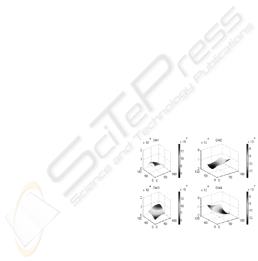
5 SINGULARITY ANALYSIS
As shown in the previous section, the linear
velocities of the actuators
l
are related to the
angular velocity of the moving platform
ω
by (28),
in which
J was the 34
×
Jacobian matrix of the
hydraulic shoulder. Singularities will occur if the
Jacobian rank is lower than three, the number of
DOF of the moving platform, or equivalently if:
0)det( =JJ
T
(41)
Such a case occurs only if the determinants of all
33
×
minors of J are identically zero. These square
minors correspond to the Jacobian matrices of the
hydraulic shoulder with one of the actuating legs
removed. Therefore, the redundant manipulator will
be in a singular configuration only if all the non-
redundant structures resulted by suppressing one of
the actuating legs are in a singular configuration.
Such a case will not occur in the workspace of the
hydraulic shoulder owing to the specific and careful
design of the mechanism (Hayward, 94). In fact, one
of the remarkable features of adding the fourth
actuator is the elimination of the loci of singularities.
Fig.(5), shows the determinants of the four minor
Jacobian matrices, computed in the workspace of the
manipulator where DM1-DM4 denote the non-
redundant minor determinants. This can be of
interest in cases where one of the actuators
malfunctions. It can be seen that the possibility of
getting into a singular configuration is increased
when either of the redundant actuators are removed.
Figure 4: Minor Determinants for the non-redundant
structures
6 CONCLUSIONS
In this paper, kinematic modeling and singularity
analysis of a 3-DOF actuator redundant parallel
ICINCO 2005 - ROBOTICS AND AUTOMATION
130

manipulator has been studied in detail. The closed
form solution to the forward kinematic is obtained
using a vector approach by considering the
individual kinematic chains inherent in such parallel
mechanisms. It is proposed to consider suitable
mapping between actuator, joint and task spaces in
both kinematic and Jacobian modeling of the
manipulator. The proposed method paves the way
for the feedback position control of the manipulator,
using a closed-form solution to the forward
kinematics and leaving out the approximation errors
inherent in numerical identification methods. It is
also shown that the forward kinematics map
provides us with some extra solutions which should
be regarded properly. Singularity analysis was also
performed using the analytic Jacobian obtained for
the mechanism. The manipulator workspace was
shown to be free of singularities due to the
redundancy in actuation. Future work will consider
Dynamic analysis of the hydraulic shoulder
manipulator.
REFERENCES
J.P. Merlet, Still a long way to go on the road for parallel
mechanisms, ASME 2002 DETC Conference,
Montreal, Canada, 2002
J.P. Merlet, Parallel Robots: Open problems, In 9th Int'l.
Symp. of Robotics Research, Snowbird, 9-12 October
1999.
S. Joshi and L.W. Tsai, The kinematics of a class of 3-
DOF , 4-Legged parallel manipulators, Trans. Of the
ASME, vol. 125, March 2003, 52-60.
S. Joshi and L.W. Tsai, A comparison study of two 3-DOF
parallel manipulators: One with three and the other
with four supporting legs, IEEE Trans. On Robotics &
Automation, vol. 19, No. 2, April 2003, 200-209.
L.Baron and J. Angeles, The kinematic decoupling of
parallel manipulators using joint-sensor data, IEEE
Trans. On Robotics & Automation, vol. 16, No. 6, Dec
2000, 644-651.
J.P.Merlet, Closed-form resolution of the direct kinematics
of parallel manipulators using extra sensors data, IEEE
Intl. Conf. On Robotics & Automation, 1993, 200-
204.
J.P.Merlet, Direct kinematics of planar parallel
manipulators, Intl. Conf. On Robotics & Automation,
Minnesota, April 1996, 3744-3749.
S.K.Song and D.S.Kwon, Efficient formulation approach
for the forward kinematics of the 3-6 Stewart-Gough
platform, Intl. Conf. on Intelligent Robots and
Systems, Hawaii, USA, Oct. 2001, 1688-1693.
Bonev, I. A., Ryu, J., Kim, S.-G., and Lee, S.-K., A
closed-form solution to the direct kinematics of nearly
general parallel manipulators with optimally located
three linear extra sensors, IEEE Trans. On Robotics &
Automation, vol. 17, No. 2, April 2001, 148-156.
B. Siciliano, The tricept robot: inverse kinematics,
manipulability analysis and closed-loop direct
kinematics algorithm, Robotica, vol. 17, pp.437-445,
June 1999.
A. Fattah and G. Kasaei, Kinematics and dynamics of a
parallel manipulator with a new architecture,
Robotica, vol. 18, pp. 535-543, Sept. 2000.
O.Didrit, M.Petitot and E.Walter, Guaranteed solution of
direct kinematic problems for general configurations
of parallel manipulators, IEEE Trans. On Robotics &
Automation, April 1998, 259-266.
B. Dasgupta, T.S. Mruthyunjaya, The Stewart platform
manipulator: a review, Elsevier Science, Mechanism
& Machine theory,2000,15-40.
Hayward, V. and Kurtz, R.: Modeling of a parallel wrist
mechanism with actuator redundancy, Int'l. J.
Laboratory Robotics and Automation, VCH
Publishers, Vol. 4, No. 2.1992, 69-76.
Hayward, V.: “Design of a hydraulic robot shoulder based
on a combinatorial mechanism” Experimental
Robotics III: The 3rd Int'l Symposium, Japan Oct.
1994. Lecture Notes in Control & Information
Sciences, Springer-Verlag, 297-310.
Hayward, V.: “Borrowing some design ideas from
biological manipulators to design an artificial one” in
Robots and Biological System, NATO Series,
Springer-Verlag, 1993, 135-148.
H. Sadjadian and H.D. Taghirad, Numerical Methods for
Computing the Forward Kinematics of a Redundant
Parallel Manipulator, IEEE Conf. on Mechatronics
and Robotics, pp 557-562, Sept. 2004, Aachen,
Germany.
KINEMATIC AND SINGULARITY ANALYSIS OF THE HYDRAULIC SHOULDER: A 3-DOF Redundant Parallel
Manipulator
131
