
A REACTIVE MOTION PLANNER ARCHITECTURE FOR
GENERIC MOBILE ROBOTS
BASED ON MULTILAYERED CELLULAR AUTOMATA
Fabio M. Marchese
Universit
`
a degli Studi di Milano - Bicocca
Via Bicocca degli Arcimboldi 8, I-20126, Milan (Italy)
Keywords:
Mobile Robots, Motion Planning, Cellular Automata, Trajectories Generation.
Abstract:
The aim of this paper is to describe the architecture of a Path Planner for Mobile Robots based on the paradigm
of Cellular Automata. The environment representation is distributed, as the robot shape; both and the robot
kinematics are parameters for the planner. Hence, it results to be very flexible, handling robots with quite
different kinematics (omnidirectional, car-like, asymmetrical, etc.), with generic shapes (even with concavities
and holes) and with generic cinematic center positions. Because of these characteristics, it is applicable for the
assembly planning in the manufacturing industry, as in the Piano Mover’s problems, or in vehicles trajectories
generation. It can be applied to flat (Euclidean) Work Space and to natural variable terrains. Considering
robots moving with smoothed trajectories, the underlying algorithm is based on a Potential Fields Method,
using an anisotropic propagation of potentials on a non-Euclidean manifold. The collision-free trajectories
are found following the minimum valley of the potential hypersurface embedded in a 4D space. Thanks to
the Multilayered Cellular Automata architecture, it turns out to be very fast, complete and optimal, allowing
to react to the wold dynamics (reactive planning), generating new optimal solutions every time the obstacles
positions changes.
1 INTRODUCTION
The work presented in this paper concerns Mobile
Robots Path-Planning exploiting Multilayered Cellu-
lar Automata (MCA). The Path-planning problem is
very important to drive mobile robots in environments
avoiding collision with obstacles. In our work, we
consider robots with different types of kinematics: for
example, robots moving thanks to differential drives
(moving forward and backward, and rotating in the
place), robots moving as cars (car-like kinematics or
non-holonomic), robots also translating in any direc-
tions and rotating (sphere-like kinematics or omnidi-
rectional), etc. To realize a path-planner able to face
with different types of motion is quite problematic.
More over, we added other constrains to this prob-
lem. When a robot moves between obstacles, its real
shape and size must be considered to avoid collisions.
It is more difficult to handle robot with asymmetrical
shapes, even with concavity, holes, etc. Most of the
works in literature treat this problem substituting the
real shape with an equivalent cylinder with the same
radius, enlarging the space occupancy. This solution
is feasible when the robot moves in wide spaces, but it
is not when considering narrow spaces, cluttered en-
vironments, etc. A further complication derives from
the geometry of the world in which the robot is sit-
uated. In a flat world, as office-like structured envi-
ronments, the geometry is quite simple: it is a planar
surface (Euclidean 2D Space) on which the robot nav-
igates. We want to face different situations, as motion
on natural terrains, where the Euclidean metric is no
more applicable. In this work we introduce the archi-
tecture of a complete optimal path-planner applicable
on robots with different shapes and kinematics op-
erating in a natural world. Because the use of the
paradigm of Cellular Automata, the approach is dis-
tributed and very fast, even on single-processor com-
puters. During the last twenty years, many authors
have proposed different solutions, based on geomet-
rical descriptions of the environment (e.g. (Lozano-
P
´
erez and Wesley, 1979; Lozano-P
´
erez, 1983)). In
the eighties, Khatib in (Kathib, 1985) first introduced
a new method for the collision avoidance problem in
a continuous space for a 6 DOF manipulator robot.
This alternative approach is less precise, but more ef-
ficient: the Artificial Potential Fields Methods. Ja-
hanbin and Fallside introduced a Wave Propagation
82
M. Marchese F. (2005).
A REACTIVE MOTION PLANNER ARCHITECTURE FOR GENERIC MOBILE ROBOTS BASED ON MULTILAYERED CELLULAR AUTOMATA.
In Proceedings of the Second International Conference on Informatics in Control, Automation and Robotics - Robotics and Automation, pages 82-87
DOI: 10.5220/0001184500820087
Copyright
c
SciTePress
algorithm in the discretized Configuration Space (C-
Space) (Distance Transform (Jahanbin and Fallside,
1988)). Barraquand et al. in 1992 (Barraquand et al.,
1992) used the Numerical Potential Field technique
on the C-Space to build a generalized Voronoi Dia-
gram. Zelinsky extended the Distance Transform to
the Path Transform (Zelinsky, 1994). Tzionas et al.
in (Tzionas et al., 1997) described an algorithm for
a diamond-shaped holonomic robot in a static envi-
ronment, where they let a CA to build a Voronoi Di-
agram. Pai and Reissel in (Pai and Reissell, 1998)
introduced a Motion Planning algorithm on multires-
olution representation of terrains using wavelets. The
path finding is based on a variation of Dijkstra’s
algorithm on a regular 2D lattice. In (Kobilarov
and Sukhatme, 2004), the authors presented a Path-
Planner for outdoor terrain based on the Control The-
ory and the technique of random trees (RRT). We used
CA as a formalism for merging the Grid Model of
the world (Occupancy Grid) with the C-Space of a ro-
bot and Numerical (Artificial) Potential Field meth-
ods, with the task to find a simple and fast solution
for the path-planning problem for mobile robots with
different kinematics. This method uses a directional
(anisotropic) propagation of distance values between
adjacent automata to build a potential hypersurface
embedded in 4D space. Using a constrained version
of the descending gradient on the hypersurface, it is
possible to find out all the admissible, equivalent and
shortest (for a given metric of the discretized space)
trajectories connecting two configurations of the ro-
bot C-Space.
2 PROBLEM STATEMENTS
A wide variety of world models can be used to de-
scribe the interaction between an autonomous agent
and its environment. One of the most important is
the Configuration Space (Lozano-P
´
erez, 1983). The
C-Space C of a rigid body is the set of all its configu-
rations q (i.e. poses). If the robot can freely translate
and rotate on a 2D surface, the C-Space is a 3D mani-
fold (R
2
×SO(2) ≡ SE(2)). It can be modelled using
Figure 1: Mobile Robot Path-Planner Architecture
a 3D Bitmap GC (C-Space Binary Bitmap), a regular
decomposition in cells of the C-Space, represented by
the application GC : C → {0, 1}, where 0s represent
non admissible configurations. The C-Potential is a
function U(q) defined over the C-Space that ”drives”
the robot through the sequence of configuration points
to reach the goal pose (Barraquand et al., 1992). Let
us introduce some other assumptions: 1) space topol-
ogy is finite and planar; 2) the robot has a lower bound
on the steering radius (non-holonomic vehicle). The
latter assumption introduces important restrictions on
the types of trajectories to be found. In the following
section, we will describe each layer and its properties.
3 THE PATH-PLANNER
ARCHITECTURE
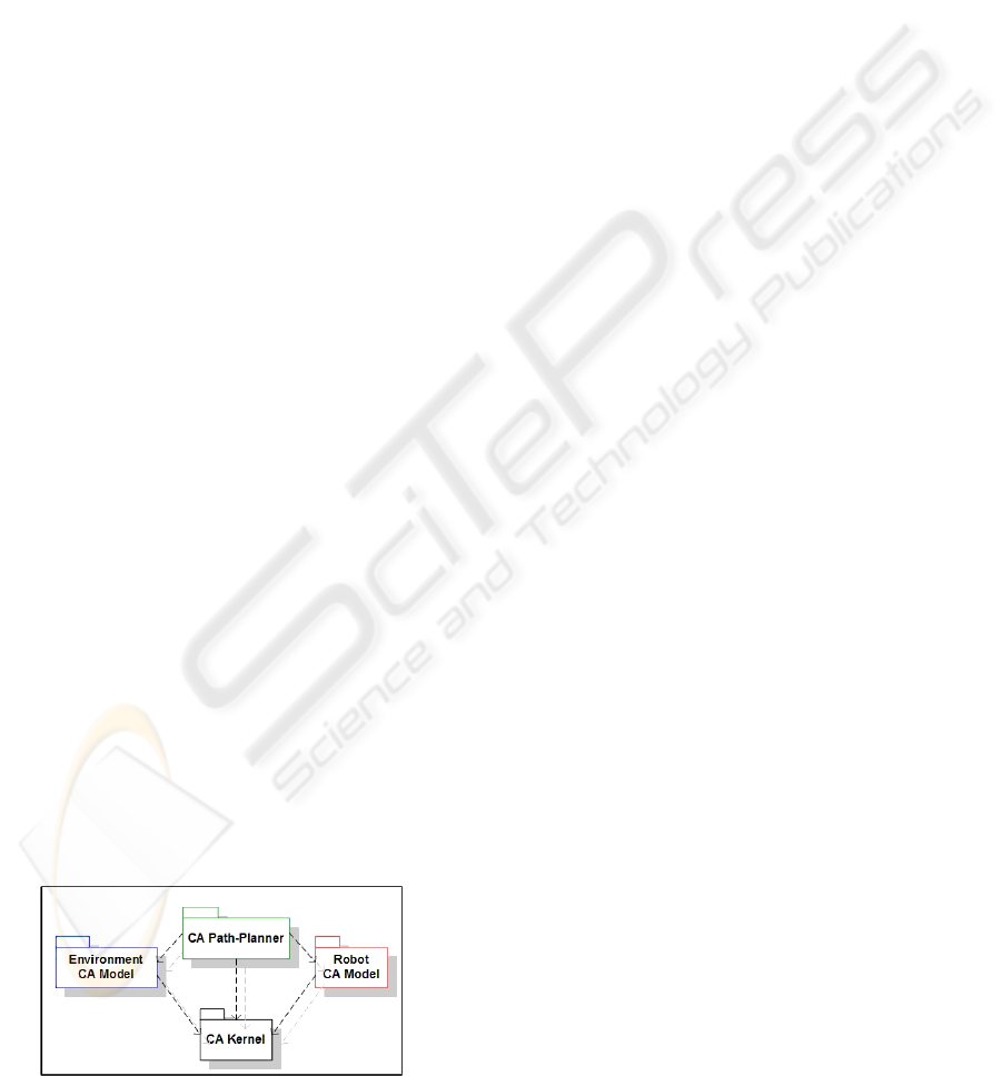
The planner architecture is organized in four main
packages (Fig. 1). The main package is the Path-
Planner itself: it coordinates the two lateral packages
(Environment and Robot Models). It is worth not-
ing that the World Model, the Robot Model and the
Path-Planner use the same structure based on Cellu-
lar Automata, i.e. there is an isomorphism based on a
regular decomposition structure.
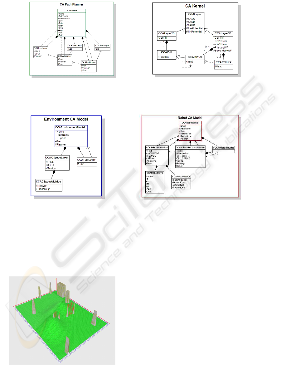
3.1 CA Kernel
The CA Kernel realizes the Cellular Automata para-
digm (Fig. 2.b). The architecture is organized in lay-
ers of cells depending on the underlying topological
space. There are bi-dimensional spaces, such as the
Work-Space, and 3D spaces (C-Space, Attraction Po-
tential, etc.); some of them are active and are used to
make calculations, others are static and are used only
to represent specific information. The package makes
available the basic structures to represent the informa-
tion of both types of spaces and the related calculation
kernel.
3.2 Environment CA Model
The Environment Model (Fig. 3.a) is subdivided in
two parts: the C-Space and the Terrain Elevation Map.
The first is a 3D space (SE(2), i.e. position and orien-
tation) in which are represented both the C-Obstacles
and the C
free
-Space. The second is a regular 2D man-
ifold representing the elevation map (z = f(x, y)) of
the terrain on which the robot navigates. In a struc-
tured world (e.g. an office-like environment), it is
simply as a flat surface (z = 0). There is space metric
associated to the C-Space. Formally, in a continuous
space, it is a set of parameters used to define a matrix
(fundamental tensor) necessary to evaluate the infini-
tesimal distance between two neighboring points. In
A REACTIVE MOTION PLANNER ARCHITECTURE FOR GENERIC MOBILE ROBOTS BASED ON
MULTILAYERED CELLULAR AUTOMATA
83
(a) (b)
Figure 2: Packages inside views (A)
(a) (b)
Figure 3: Packages inside views (B)
our case, the space is discretized in cells (CA), and
the set of parameters are slightly different, but the has
the same role: the evaluation of the linear distance
between two adjacent cells in the 3D C-Space.
Figure 4: An example of Environment Model as a combi-
nation of Terrain and Obstacles Layers
3.3 Robot CA Model
This package is used to model the robot (Fig. 3.b).
Two major components are necessary to model the
robot: its shape and its kinematics. The shape is de-
fined using a 2D CA (Fig. 5.a): it is a small occupancy
map centered on the robot cinematic center. The ro-
bot kinematics is defined as a set of available moves.
Each move allows the robot to rototranslate from the
current cell to an adjacent one. The kinematics de-
finition is completed with a robot metric. This is a
set of costs associated to each robot move, to evalu-
ate the cost (in term of energy or time or path length)
the robot has to spend to reach a new pose. From this
two structures is derived a secondary structure con-
taining the Motion Silhouettes. In Regular Decom-
position world models, the obstacles are decomposed
in full or empty cells (Occupancy Grids) and the ro-
bot is shrunk to a point (the robot cinematic center).
The well-known technique of enlarging the obstacles
by the robot maximum radius is then used to take into
account of its real extension (Lozano-P
´
erez and Wes-
ICINCO 2005 - ROBOTICS AND AUTOMATION
84
ley, 1979). An isotropic enlargement with a constant
radius would give the same results as using an equiva-
lent cylindrical robot. The consequence is a great loss
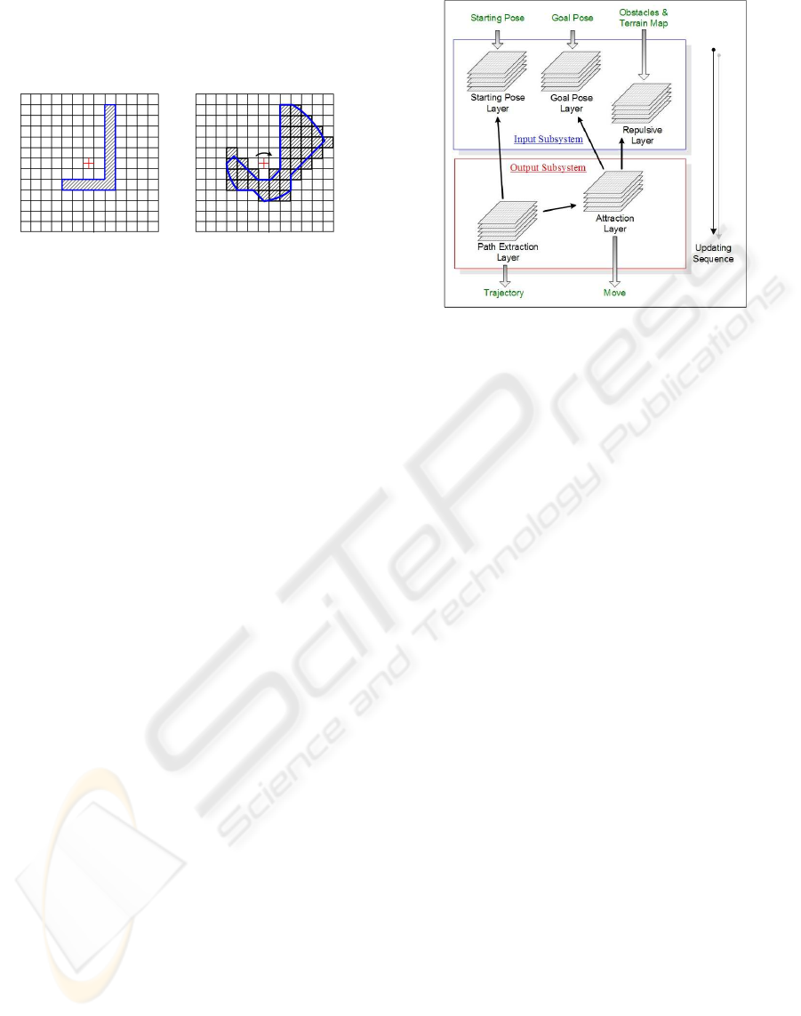
(a) (b)
Figure 5: An example of CA silhouette for a L-shaped ro-
bot (red cross: cinematic center): a) basic silhouette (robot
shape); b) a motion silhouette obtained sweeping the robot
silhouette during a single movement (rotation)
of space around the obstacles, and many trajectories
are lost. An anisotropic enlargement (Lozano-P
´
erez
and Wesley, 1979), i.e. a different obstacles enlarge-
ment for each robot orientation, would solve only par-
tially the problem for asymmetric robots. Counter-
examples can be shown where the robot still collides
with obstacles between two consecutive poses. We
adopted a different approach to address this problem,
by defining the Motion Silhouettes (e.g. Fig. 5.b)
and evaluating cell by cell the set of admissible ro-
bot movements that avoid collisions (see Repulsive
Layer in 3.4.1). The Motion Silhouette is generated
by sweeping the basic robot shape during a single
move and marking the cells covered. To avoid col-
lisions, there must not be any obstacles cells in the
marked cells. The Motion Silhouettes are calculated
off-line once for all for any robot orientation, combin-
ing the set of movements (robot kinematics) and the
basic silhouette (robot shape).
3.4 CA Path-Planner
The Path-Planner of Fig. 2.a is a sort of ”bridge” be-
tween the Environment Model and the Robot Model.
It combines the information from both to generate a
set of optimal trajectories. It is organized in two ma-
jor subsystems: an Input Subsystem and an Output
Subsystem (Fig. 6). They are subdivided in five sub-
layers (3 + 2), some of them are statical and the others
evolve during the planning time. The Input Subsys-
tem is an interface toward the outstanding environ-
ment. Its layers have to react as fast as possible to
the external changes: the robot starting pose, the ro-
bot goal pose, the elevation map of the terrain and,
the most important, the changes of the environment,
i.e. the obstacles movements in a dynamic world.
The first two layers (Starting Pose L. and Goal Pose
Figure 6: Path-Planner Layers Structure
L. are considered quasi-statical, because they are up-
dated from the outside at a very low frequency (much
lower than the internal updating frequency); the Re-
pulsive L. is updated externally (by means of a per-
ception system) and it evolves testing the robot move-
ments admissibility to avoid collisions. The Output
Subsystem returns the results of the planning, that is
the set of complete trajectories from the Path Extrac-
tion L., or a single motion step from the Attraction L.
3.4.1 Repulsive Layer
The Repulsive Layer is the dynamical version of the
C-Space. It is first initialized with the C-Obstacles in
the Environment CA Model, then it starts evolving to
find out cell by cell any admissible move (Collision-
free Moves) exploiting the Motion Silhouettes previ-
ously determinated. The admissibility of a move is
influenced: 1) globally, by the specific robot kinemat-
ics; 2) locally, by the vicinity of an obstacle and by
the robot shape. This layer is decomposed in sub-
layers, one for each robot orientation and move: it is
itself a Multilayered CA on a 2D domain (the space
R
2
of positions). It is a particular type of Cellular Au-
tomata also for another reason: the cell neighborhood
does not have the standard square shape, but a non-
standard fixed architecture (Sipper, 1997). Its par-
ticular shape reflects the robot Motion Silhouette as
shown in the example of Fig. 5.b. In Fig. 7 is shown
the result of the evolution of this layer for a rectangu-
lar robot using the terrain of Fig. 4.b. The grey level
is proportional to the number of admissible moves,
ranging from white (all moves admissible) to black
(no move).
A REACTIVE MOTION PLANNER ARCHITECTURE FOR GENERIC MOBILE ROBOTS BASED ON
MULTILAYERED CELLULAR AUTOMATA
85
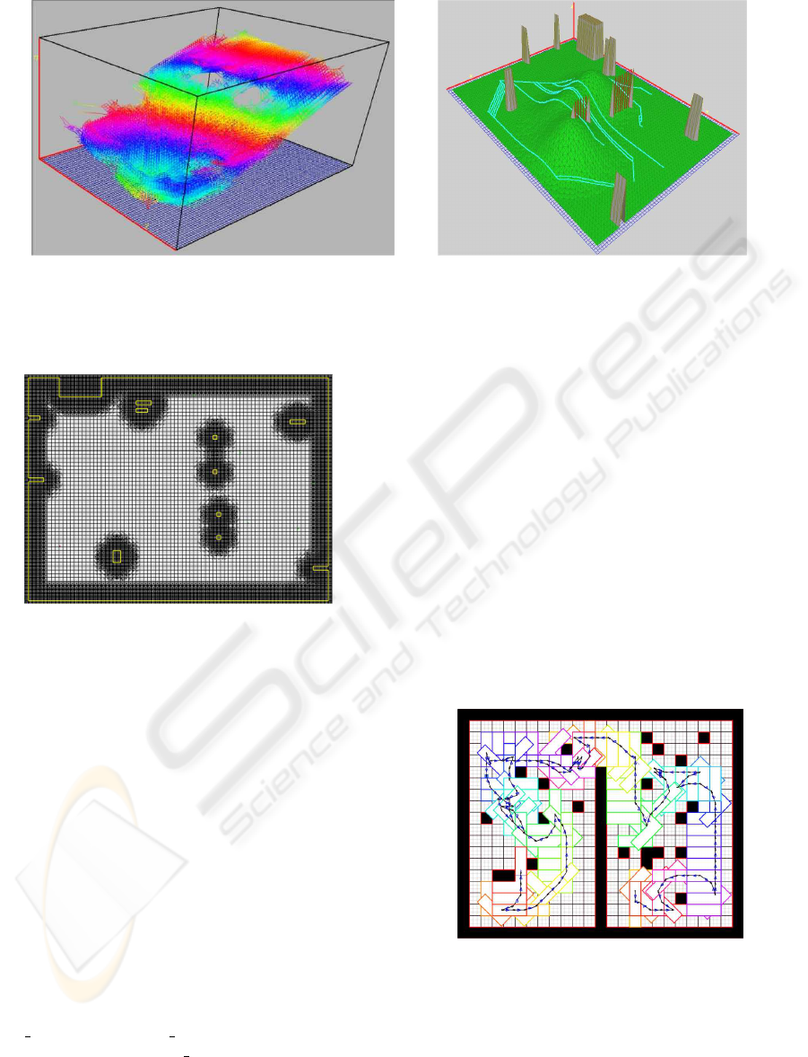
(a) (b)
Figure 9: An example with a car-like robot: a) Attraction Potentials hypersurface (3D skeleton); b) Trajectories on the
elevation map;
Figure 7: An example of the Obstacles Layer for a rectan-
gular Robot moving in Fig. 4 world
3.4.2 Attraction Layer
This layer is the main part of the entire Path-Planning
Algorithm. The Attraction Layer is the digitalized
representation of the C-Potential function U(q) de-
fined on the C-Space Bitmap: for any position and
orientation is calculated a potential value. The C-
Potential is a potential surface with a global minimum
in the goal cell. The potential represents the inte-
ger ”distance” of the cell c from the Goal cell when
the robot moves with an outgoing direction along a
collision-free path, or more simply it is the cost to
reach the goal from the cell c. To evaluate the path
cost, we have introduced the Robot Metric as a set
of costs for the basic robot movement: (forward, for-
ward
diagonal, direction change, stop, rotation, lat-
eral, backward, backward
diagonal). These basic
movements are combined in different ways to repre-
sent the different robots kinematics. The robot can
be subjected also to non-holonomic constraints, there-
fore not every movement can be done as an omnidi-
rectional robot does. To treat different kinematics, we
have introduced a subset of admissible moving direc-
tions (D
′
(c, d) ⊆ D) depending on the robot posi-
tion (cell c) and orientation d compiled off-line on the
base of the robot kinematics. Changing the metric,
we can realize the kinematics of different robots. For
example, the kinematics (2, 3, 1, 0, High, High, 2, 3)
emulates a common car-like kinematics (Reed’s and
Shepp’s vehicle), while A robot also translating in
any direction (omnidirectional) has a kinematics like:
(2, 3, 1, 0, 1, 2, 2, 3). To compute the path length, an
Environment Metric (3.2) is needed. On a flat environ-
ment (Euclidean Space), the distance between cells
(the space metric) is invariant with respect to the po-
sition. For variable terrains, the cost value must de-
Figure 8: Manoeuvering example for a L-robot in a clut-
tered world
pend on the 3D distance between points on the sur-
face, on the difference of elevation between two po-
sitions, hence the space metric changes from point
to point. For this reason, it is necessary to include
the surface gradient in the cost function. The over-
ICINCO 2005 - ROBOTICS AND AUTOMATION
86

all path cost results in a combination of robot met-
ric, environment metric and surface gradient (a kind
of ”path-planner metric”). Two main properties can
be demonstrated: the termination of the propagation
of the potential values through the C-Space and the
absence of local minima. The later property ensures
to achieve the goal (in the global minimum) just fol-
lowing the negated gradient vector of the C-Potential
function without stalling in any local minima.
4 EXPERIMENTS AND RESULTS
We have generated some synthetic elevation maps and
introduced an obstacle distribution to observe the al-
gorithm behavior. An interesting property of this al-
gorithm is the simultaneous computation of trajecto-
ries from more than one starting position. We exploit
this property to show multiple problems in the same
environment. In the example of Fig. 9, the terrain has
a group of three ”hills” in the middle, and we con-
sider five different starting points of the robot and one
goal (bottom-left). From any position, the robot tries
to move around the hills, unless the shortest path is
to pass over them (in any case, at the minimum ele-
vation). The performance tests, carried out with an
Intel Pentium IV 2.26 GHz PC, gave the following
result (mean times over 500 repetitions ): 182 ms
(Fig. 9), 26.7 ms (Fig. 8). The complexity of a path-
planning algorithm is always strictly related to the ob-
stacles distribution. A good upper-bound estimate, in
the worst cases without obstacles enlargements, can
be done. Considering that the longest paths cover ap-
proximatively 1/2 of the total number of cells N of
the 2D Workspace Bitmap, and require nearly 2
N
2
N
cells updates to be computed, a realistic upper-bound
of the complexity is O(N
2
). If we take also into ac-
count of the obstacles enlargements, the result is even
better since the number of free cells is much lower,
especially in a cluttered world.
5 CONCLUSION
In this paper we have described an architecture solu-
tion for the Path-Planning Problem for mobile robots
with generic shapes (user defined) and with generic
kinematics on variable (regular) terrains based on
(Multilayered) Cellular Automata. Another impor-
tant property of this algorithm is related to the con-
sistency of the solution found. For a given terrain sur-
face, the solution found (if it exists) is the set of all
shortest paths (for the given metric) that connect the
starting cell to the goal cell. The CA evolution can be
seen as a motion from one point to another point of a
global state space until an optimal solution is reached.
This is a convergence point for the given problem or
a steady global state. If we make some perturbations,
such as changing the environment (e.g. adding, delet-
ing or moving one or more obstacles), then the point
becomes unstable and the CA starts to evolve again
towards a new steady state, finding a new set of opti-
mal trajectories (Incremental Updating).
REFERENCES
Barraquand, J., Langlois, B., and Latombe, J. C. (1992).
Numerical potential field techniques for robot path
planning. IEEE Trans. on Systems, Man and Cyber-
netics, 22(2):224–241.
Jahanbin, M. R. and Fallside, F. (1988). Path planning us-
ing a wave simulation technique in the configuration
space. In Artificial Intelligence in Engineering: Ro-
botics and Processes (J. S. Gero ed.), Southampton.
Computational Mechanics Publications.
Kathib, O. (1985). Real-time obstacle avoidance for ma-
nipulator and mobile robots. In Int. Conf. on Robotics
and Automation.
Kobilarov, M. and Sukhatme, G. S. (2004). Time optimal
path planning on outdoor terrain for mobile robots un-
der dynamic constraints. In IEEE/RSJ Int. Conf. on
Intelligent Robots and Systems.
Lozano-P
´
erez, T. (1983). Spatial planning: A configura-
tion space approach. IEEE Trans. on Computers, C-
32(2):108–120.
Lozano-P
´
erez, T. and Wesley, M. A. (1979). An algo-
rithm for planning collision-free paths among polyhe-
dral obstacles. Comm. of the ACM, 22(10):560–570.
Pai, D. K. and Reissell, L. M. (1998). Multiresolution rough
terrain motion planning. IEEE Trans. on Robotics and
Automation, 14(1):19–33.
Sipper, M., editor (1997). Evolution of Parallel Cellular
Machines - The Cellular Programming Approach, vol-
ume 1194 of LNCS. Springer-Verlag.
Tzionas, P. G., Thanailakis, A., and Tsalides, P. G. (1997).
Collision-free path planning for a diamond-shaped ro-
bot using two-dimensional cellular automata. IEEE
Trans. on Robotics and Automation, 13(2):237–250.
Zelinsky, A. (1994). Using path transforms to guide the
search for findpath in 2d. Int. J. of Robotics Research,
13(4):315–325.
A REACTIVE MOTION PLANNER ARCHITECTURE FOR GENERIC MOBILE ROBOTS BASED ON
MULTILAYERED CELLULAR AUTOMATA
87
