
OPTIMIZED FUZZY SCHEDULING OF MANUFACTURING
SYSTEMS
N. C. Tsourveloudis, L. Doitsidis
Department of Production Engineering and Management, Technical University of Crete,
Chania 73100,Greece
S. Ioannidis
Department of Mathematics, University of the Aegean, Samos, Greece
Keywords: Work-In-Process, Backlog, Fuzzy Scheduling, Evolutionary Algorithms, Manufacturing Systems.
Abstract: An Evolutionary Algorithm (EA) strategy for the optimization of generic Work-In-Process (WIP)
scheduling fuzzy controllers is presented. The EA is used to tune a set of fuzzy control modules which are
used for distributed and supervisory WIP scheduling. The distributed controllers objective is to control the
rate in each production stage so that satisfies the demand for final products while reducing WIP within the
system. The EA identifies the parameters for which the fuzzy controller performs optimal with respect to
WIP and backlog minimization. The proposed strategy is compared to known heuristically tuned fuzzy
control approaches. Simulation results show that the EA strategy improves system’s performance.
1 INTRODUCTION
The Work-In-Process (WIP) inventory is measured
by the number of unfinished parts in the buffers
throughout the manufacturing system. For various
reasons reported in (Conway et al, 1998) and
elsewhere, the in-process inventories should stay as
small as possible. The important question in WIP
management is: what is the minimum necessary
WIP? The answer, which is not straightforward, is
that WIP is highly associated with the fluctuations of
demand. WIP is accumulated when the actual
production rate is higher than the demand. However,
when WIP is very low, unpredicted phenomena,
such as machine failures, may lead the actual
production behind the demand and thus to delayed
deliveries and unsatisfied customers. Obviously,
product demands of constant level and pattern make
scheduling easier than randomly changing demands.
Control policies that tend to keep WIP in low
levels have drawn a great deal of attention from
researchers and practitioners (Gershwin et al, 1994),
(Bai et al, 1994). Recently, artificial intelligence-
based methodologies for the WIP control of realistic
(in terms of modelling assumptions) manufacturing
systems have been presented ((Tsourveloudis et al
2000),(Ioannidis et al, 2004), (Custodio et al, 1994)).
In previous work ((Tsourveloudis et al 2000),
(Ioannidis et al, 2004)), distributed and supervisory
schemes for the control of WIP where introduced. In
both approaches presented the controllers performed
better from traditional and surplus-based policies.
However, neither this approach has adopted a
systematic methodology that ensures optimal design
of the in – process inventory controllers.
In this paper we present an Evolutionary
Algorithm (EA) strategy for optimization of generic
WIP scheduling fuzzy controllers introduced in
(Tsourveloudis et al 2000), (Ioannidis et al, 2004).
The scheduling problem objective is to control the
production rate in a way that satisfies the demand for
final products while keeping minimum WIP within
the production system. During the evolution, the EA
identifies those set of parameters for which the fuzzy
controller performs optimal with respect to WIP
minimization for several demand patterns.
2 FUZZY SCHEDULING
A production system can be viewed as a network of
machines and buffers. Items are received at each
machine and wait for the next operation in a finite
capacity buffer. The machines break down randomly
and may be incapable of producing more parts
196
C. Tsourveloudis N., Doitsidis L. and Ioannidis S. (2005).
OPTIMIZED FUZZY SCHEDULING OF MANUFACTURING SYSTEMS.
In Proceedings of the Second International Conference on Informatics in Control, Automation and Robotics, pages 196-201
DOI: 10.5220/0001184401960201
Copyright
c
SciTePress
B
j,i
B
i,l
M
i
because of starvation and/or blocking phenomena.
Due to a failed machine with operational neighbors,
the level of the downstream buffer decreases, while
the upstream increases. If the repair time is big
enough, then the broken machine will either block
the next station or starve the previous one. This
effect will propagate throughout the system.
Clearly, production scheduling of realistic
manufacturing plants must satisfy multiple
conflicting criteria and also cope with the dynamic
nature of such environments. Fuzzy logic offers the
mathematical framework that allows for simple
knowledge representations of the production control
/ scheduling principles in terms of IF-THEN rules.
Two approaches of production scheduling have
been identified, the distributed and the supervisory
fuzzy scheduling. The advantage of the fuzzy
controllers used in the distributed approach is that
computationally simple and therefore facilitate
application to real time control/scheduling.
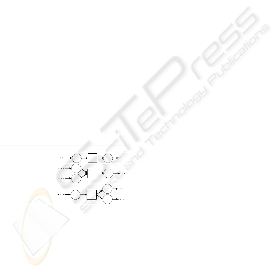
In the distributed fuzzy scheduling system
presented in (Tsourveloudis et al, 2000), three basic
subsystems have been introduced, namely transfer
line, assembly and disassembly module. The
majority of the real production networks can be
decomposed into these subsystems. Each subsystem
can be seen as a distributed fuzzy logic controller.
The inputs of the control modules (Table 1) are
the buffer levels B
ji
, B
il
,
B
ki
, B
ik
, B
il
, the state s
i
of the
machine M
i
, the production surplus x
i
of M
i
and the
sole output is the processing rate r
i
of M
i
.
Table 1: Control Modules
Module Schema
Line
Assembly
Disassembly
The control objective of the distributed
scheduling approach, is to satisfy the demand keep
WIP as low as possible. This is attempted by
regulating the processing rate r
i
at every time instant.
The expert knowledge that describes the control
objective can be summarized as follows:
If the surplus level is satisfactory then try to
prevent starving or blocking by increasing or
decreasing the production rate accordingly.
If the surplus is either too low or too high then
produce at maximum or zero rate respectively.
The above knowledge is formally represented,
for the control modules of Table 1, by fuzzy rules. In
the case of the transfer line rule has the form:
IF b
j,i
is LB
(k)
AND b
i,l
is LB
(k)
AND s
i
is LS
i
(k)
AND x
i
is LX
(k)
THEN r
i
is LR
i
(k)
where k is the rule number, i is the number of
machine or workstation, LB is a linguistic value of
the variable buffer level b with term set B= {Empty,
Almost Empty, OK, Almost Full, Full}, s
i
denotes the
state of machine i, which can be either 1 (operative)
or 0 (stopped); consequently S= {0, 1}. LX
represents the value that surplus x takes and it is
chosen from the term set X= {Negative, OK,
Positive}. The production rate r takes linguistic
values LR from the term set R= {Zero, Low, Almost
Low, Normal, Almost High, High}. The processing
rate r
i
of each machine at every time instant is
⎪
⎩
⎪
⎨
⎧
=
=
==
′
∑
∑
∗
∗
1
)(
)(
00
),,,(
,,
i
iR
iRi
i
iiliijisi
sif
r
rr
sif
sxbbfr
µ
µ
, (1)
where,
),,,(
,, iiliijis
sxbbf represents a fuzzy
inference system ([7], [8]) that takes as inputs the
level b
j,i
of the upstream buffer, the downstream
buffer level b
i,l
, x
i
is the surplus (cumulative
production minus demand) and s
i
is a non fuzzy
variable denoting the state of the machine, which
can be either 1 (operative) or 0 (stopped). In (1),
)(
iR
r
∗
µ
is the membership function of the aggregated
production rate, which is given by
)],,,(
),,,([minmax)(
,,
,,
,,
)(
,,
iiliij
FR
iliijAND
xbb
iR
rxbb
xbbr
k
iliij
µ
µµ
∗∗
=
, (2)
where
),,(
,,
*
iliijAND
xbb
µ
is the membership function
of the conjunction of the inputs and
),,,(
,,
)(
iiliij
FR
rxbb
k
µ
is the membership function of
the k-th activated rule. That is
)()()(),,(
,,,, iXliBijBiliijAND
xbbxbb
∗∗∗∗
∧∧=
µµµµ
, (3)
]
[
)(),(
),(),(),,,(
)()(
)()()(
,,,,
i
LR
i
LX
li
LB
ij
LB
iiliij
FR
rx
bbrxbb
kk
kkk
f
µµ
µµµ
→
=
, (4)
In equations (3), (4),
)(
,ijB
b
∗
µ
and )(
,liB
b
∗
µ
are
the membership functions (MFs) of the actual
upstream and downstream buffer levels and
)(
iX
x
∗
µ
is the membership function of production surplus.
In the supervised fuzzy scheduling approach, the
supervisory controller utilizes macroscopic data of
higher hierarchies to adjust the overall system's
behavior. Potentially, this may happen by modifying
the lower level controllers in a way to ultimately
achieve desired specifications. The supervisory
controller’s task, introduced in (Ioannidis et al,
2004) and its optimization discussed in the next
paragraph, is the tuning of the previously presented
B
j,i
B
k,i
M
i
B
i,l
B
j,i
M
i
B
i,l
B
i,k
OPTIMIZED FUZZY SCHEDULING OF MANUFACTURING SYSTEMS
197

distributed fuzzy controllers, in a way that improves
certain performance measures without causing a
dramatic change in the control architecture. The
overall scheduling approach remains modular since
the production control modules are not modified but
tuned by the additional supervisory controller.
In the supervisory scheduling scheme it is
assumed that the demand and the cumulative
production are known. This is important for the
production surplus monitoring and control and for
scheduling decisions based on production surplus.
The expert knowledge that describes the supervisory
control objective builds on the assumption that
adaptive surplus bounds may improve the
production systems performance and can be
summarized in the following statements:
If the upper surplus bound is reduced there is an
immediate reduction of WIP.
If the upper surplus bound is increased there is
an increase of WIP and the total production rate
leading to a small reduction of backlog.
If the lower surplus bound is increased a
substantial reduction of backlog and an increase in
WIP is achieved.
If there is a reduction of lower surplus bound as
a result we have a deterioration of backlog with an
improvement of WIP.
Surplus bounds are decided by the output of IF-
THEN rules of the following form:
IF mx
e
is LMX
(k)
AND e
x
is LE
x
(k)
AND e
w
is
LE
w
(k)
THEN u
c
is LU
c
(k)
AND l
c
is LL
c
(k)
,
where, k is the rule number, mx
e
is the mean surplus
of the end product, LMX is a linguistic value of the
mx
e
with term set MX= {Negative Big, Negative
Small, Zero, Positive Small, Positive Big}, e
x
is the
error of end product surplus (the difference between
surplus x
e
and the lower bound of surplus), with
linguistic value term set E
x
= {Negative, Zero,
Positive}. The relative deviation of WIP is denoted
e
w
and LE
w
is the linguistic value chosen from the
term set E
w
= {Negative, Zero, Positive}. The upper
surplus bound correction factor u
c
takes linguistic
values LU
c
from U
c
= {Negative, Negative Zero,
Zero, Positive Zero, Positive} and the lower surplus
bound correction factor l
c
takes linguistic values LL
c
from the term set L
c
= {Negative, Negative Zero,
Zero, Positive Zero, Positive}.
The crisp arithmetic values,
*
c
u
and
*
c
l
, of the
corrections of the upper and lower surplus bounds,
respectively, are given by the following
defuzzification formulas:
∑
∑
⋅
=
)(
)(
*
*
*
cU
cUc
c
u
uu
u
c
c
µ
µ
, (5a)
∑
∑
⋅
=
)(
)(
*
*
*
cl
cLc
c
u
ll
l
c
c
µ
µ
, (5b) (5a) (5a)
where
)(
*
cU
u
c
µ
and
)(
*
cL
l
c
µ
are the MFs of the upper
and lower surplus bounds, respectively. These MFs
represent the aggregated outcome of the fuzzy
inference procedure. The correct selection of input
and output membership functions characterizes the
performance of the overall scheduling task.
Since the form of the fuzzy rules of both the
distributed and supervised approach for fuzzy
scheduling have been identified, a crucial point is
the selection of the MFs. The correct choice of the
MFs is by no means trivial but plays a crucial role in
the success of an application. Consequently, the
selection of MFs if not based on a systematic
optimization procedure cannot guarantee minimum
WIP level. This is the main drawback of the
heuristic selection of MFs in case of known (or
almost known) demand patterns. The evolutionary
algorithm developed and explained in the next
section, creates MFs that fit best to scheduling
objectives. In this context, the design of the fuzzy
controllers (distributed or supervisory) can be
regarded as an optimization problem in which the set
of possible MFs constitutes the search space.
3 EVOLUTIONARY FUZZY
SCHEDULING
The use of evolving genetic structures for the
production scheduling problem, has recently gained
a lot of acceptance for the automated and optimal
design of fuzzy logic systems (Tedford et al, 2001).
Here, we consider the application of an evolutionary
algorithm for the optimal selection of MFs.
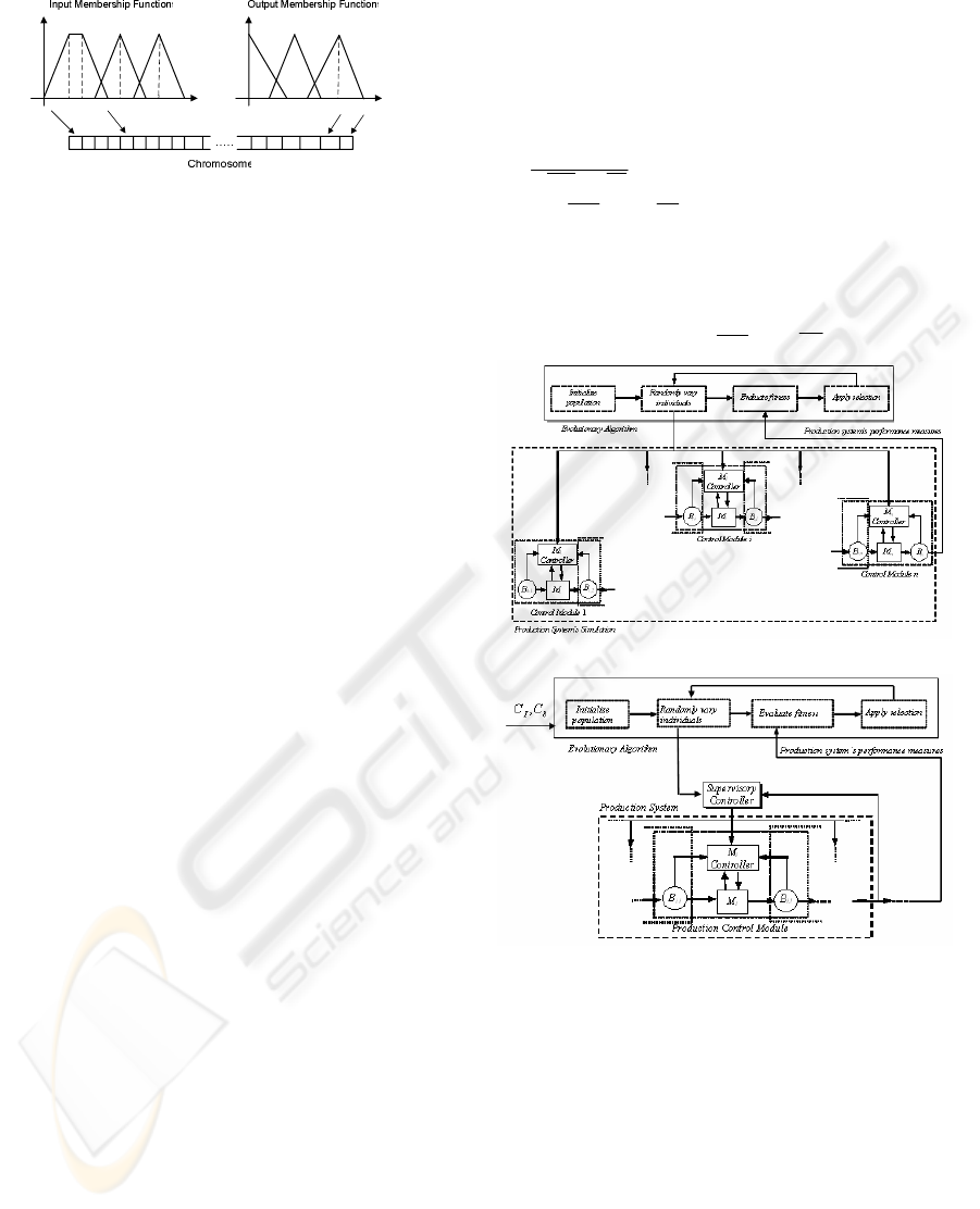
The MF defined in the previous paragraphs are
used to construct the chromosome. The basic idea is
to represent the complete set of MFs by an
individual (chromosome) and to evolve shape and
location of the MFs. This is shown in Figure 1 for
the case of trapezoidal and triangular MFs. An initial
population is derived from the first chromosome by
repeated application of the mutation operator. The
objective is to optimize a performance measure
which in the EAs context is called fitness function.
In each generation, the fitness of every chromosome
is first evaluated based on the performance of the
production network system which is controlled
through the membership functions represented in the
chromosome. A specified percentage of the better
fitted chromosomes, is retained for next generation.
Parents are selected repeatedly from the current
chromosomes generation, and new chromosomes are
generated from the parents. One generation ends
when the number of chromosomes for the next
ICINCO 2005 - INTELLIGENT CONTROL SYSTEMS AND OPTIMIZATION
198
generation has reached the quota. This process is
repeated for a pre-selected number of generations.
1
a
2
a
3
a
4
a
5
a
1
a
2
a
3
a
4
a
5
a
6
a
6
a
7
a
7
a
8
a
8
a
9
a
9
a
10
a
10
a
n
a
n
a
1−n
a
1−n
a
2−n
a
2−n
a
Figure 1: Chromosome created by the MFs
The structure of the distributed fuzzy logic
controllers as far as it concerns the rule base and the
linguistic variables remains the same with those
described in Section 2. The controllers used for
training have randomly created membership
functions. The initial population is consisted of
individuals which have the same initial chromosome
which contains the points a
i
, (i=1,…, n) that define
the membership functions of the inputs and the
output of the controllers. In case of more than one
controller the chromosome consists of the points that
define all membership functions of these controllers.
the membership functions, which correspond to the
linguistic variables, are randomly created in the
begging of the evolution process.
The evolutionary algorithm maintains a
population of individuals in each generation /
iteration. Individuals represent a different set of
distributed fuzzy controllers. In every generation the
individuals are sorted from the best to the worst
based on their fitness score. As far as it concerns the
fitness function, in the case of the distributed fuzzy
control evolution concept, it has the following form:
1
1
2
))()(()(
−
=
⎥
⎦
⎤
⎢
⎣
⎡
−=
∑
N
j
jji
tPRtDxF
, (6)
where, t is the current simulation time, T is the total
simulation time and D(t) is the overall demand and
PR(t) is the cumulative production of the system.
The architecture of the distributed evolution scheme
is presented in Figure 2.
The best individual is considered the one with
the biggest fitness. The fittest individuals are
selected and undergo mutations. The fittest
controllers and their mutated offsprings are forming
the new population. After some generations the
algorithm converges and the best individuals
represent near optimal solutions. After the evolution
process the membership functions shape is altered.
In case of the supervisory fuzzy evolutionary
scheduling, the procedure is similar. In the lower
control level were used the heuristic fuzzy
distributed controllers introduced in (Tsourveloudis
et al, 2000). The parameters were chosen as in the
distributed case, that is, population number is 40 and
mutation rate is 0.1. From the overall population the
20 fittest individuals are qualified for the next
generation while the rest are replaced by mutation of
the fittest. Each individual is evaluated by the results
of a simulation run of 200 time units. The
architecture of the supervisor evolution scheme is
shown in Figure 3.
In the case of the fuzzy supervisory evolutionary
concept the fitness function is:
BLcWIPc
F
bI
+
=
1
, (7)
where,
WIP
and
BL
are the mean work-in-process
and mean backlog, respectively. The c
I
, c
b
are
weighting factors that represent the unit costs of
inventory and backlog respectively. By taking into
account these costs in the fitness function we may
adjust the importance of
WIP
and
BL
.
Figure 2: Distributed fuzzy evolutionary concept
Figure 3: The fuzzy supervisory evolutionary concept
4 EXPERIMENTAL RESULTS
We have used the evolutionary algorithm presented
to optimize the performance of the unsupervised /
distributed and the supervised production control
schemes. The evolutionary fuzzy approaches are
tested and compared with the heuristic approaches
introduced in (Tsourveloudis et al, 2000), (Ioannidis
et al, 2004). We assume continuous parts flow
within the system. In the continuous-flow simulation
the discrete production is approximated by the
production of a liquid item (Kouikoglou et al, 1997).
OPTIMIZED FUZZY SCHEDULING OF MANUFACTURING SYSTEMS
199
Several assumptions were made for all simulations.
Machines fail randomly with a failure rate p
i
and are
repaired randomly with rate rr
i
. Unlimited repair
personnel is assumed. Time to failure and time to
repair are exponentially distributed. Demand is
either constant or stochastic with rate d. In stochastic
case it follows the Poisson distribution. Machines
operate at known, but not necessarily equal rates.
Each machine produces in a rate r
i
≤ µ
i
, where µ
i
is
the maximum processing rate of machine M
i
. The
initial buffers are infinite sources of raw material
and so the initial machines are never starved. Buffers
between adjacent machines M
i
, M
j
have finite
capacities. Set-up times or transportation times are
negligible or are included in the processing times.
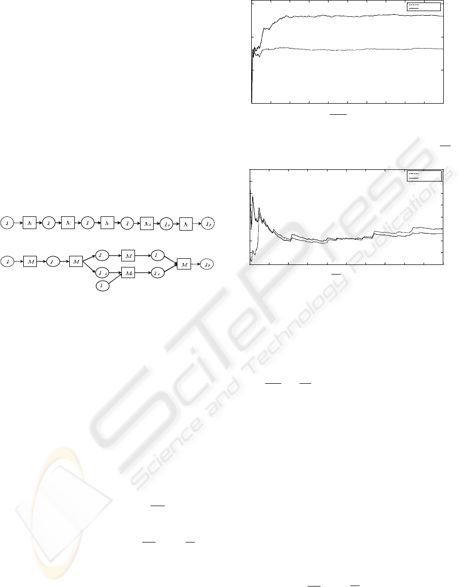
In order to test both the distributed and the
supervised evolutionary fuzzy approach the systems
presented in figures 4, 5 were used.
Figure 4: Production line
Figure 5: Production Network
4.1 Distributed evolutionary fuzzy
approach
Several scenarios have been studied for the case of
the Evolutionary Distributed Fuzzy (EDF) approach
and the results were compared with the ones
produced from the Heuristic Distributed Fuzzy
approach (HDF).
For the case of the production line, the system
under consideration consists of five machines
producing one product type. The failure and repair
rates are equal for all machines. The repair rates are
rr
i
=0.5 and the failure rates are p
i
= 0.1. The
processing rates are also equal for all machines and
are equal to µ
i
= 2 (i=1,...,5).
In Figure 6 the evolution
WIP
for both
evolutionary and heuristic systems in a simulation
run of 10000 time units is presented.
Comparative results for the
WIP
and
BL
for
various demand patterns are shown in Table 2. All
buffer capacities are equal to BC
i
= 10.
0 1000 2000 3000 4000 5000 6000 7000 8000 9000 10000
0
5
10
15
Time
Mean WIP
Evolutionary
Heuristic
Figure 6: Evolution of WIP in the production line with
stochastic demand (
d = 1)
In Figure 7 the evolution of mean backlog
BL
for the same case is presented.
0 1000 2000 3000 4000 5000 6000 7000 8000 9000
1
00
00
0
1
2
3
4
5
6
7
8
Time
Mean Backlog
Evolutionary
Heuristic
Figure 7: Evolution of
BL
in the production line with
stochastic demand (
d = 1)
The production cost consists of inventory and
backlog costs. Inventory costs are due to the capital
invested for the purchase of raw material and the
handling of material during the production process.
It is assumed that inventory cost is independent from
the stage of process. Thus, the mean production cost
C is given by:
BLcWIPcC
bI
+=
, (8)
where c
I
, c
b
are the unit costs of inventory and
backlog respectively.
The cost analysis results for the production line
examined in test case for stochastic demand are
presented in Table 3, where the production cost of
the EDF control approach is compared with the HDF
approach for various values of c
I
and c
b
. The
distributed approach was also tested in the
production network presented in Figure 6. The
production system under consideration consists of
five machines producing one part type. The failure
and repair rates of all machines are equal. The repair
rates are rr
i
= 0.5 and the failure rates are p
i
= 0.1.
The processing rates are also equal for all machines
and are equal to µ
i
= 5 (i=1,...,5). All buffer
capacities are equal to BC
i
= 10. Comparative
results for the
WIP
and
BL
for various demand
patterns are shown in Table 4.
ICINCO 2005 - INTELLIGENT CONTROL SYSTEMS AND OPTIMIZATION
200

Table 2: Results for the test case of the production line
HDF
EDF
Demand
PIW
BL
PIW
BL
Constant 1 11.492 1.72 6.371 1.567
0.5 19.393 0.057 6.417 0.438
Stochastic
1 12.719 2.496 8.07 2.427
Table 3: Cost analysis
Cost C
Demand c
I
c
b
HDF EDF
0.99
0.01
19.2
6.357
0.75
0.25
14.56
4.922
0.5
0.5
9.725
3.428
0.25
0.75
4.891
1.933
0.5
0.01
0.99
0.25
0.498
0.99
0.01
12.617
8.014
0.75
0.25
10.163
6.659
0.5
0.5
7.608
5.249
0.25
0.75
5.052
3.834
1
0.01
0.99
2.598
2.483
Table 4: Results for the production network test case
HDF
EDF
Demand
PIW
BL
PIW
BL
Constant 1 21.356 0.078 16.542 0.737
0.5
20.097
0.049
17.34
0.136
Stochastic
1
20.496
0.087
10.046
0.673
4.2 Supervised fuzzy evolutionary
approach
The Evolutionary Supervised Fuzzy approach (ESF)
was tested in the case of the production line of the
Figure 4 and was compared with the Heuristic
Supervised Fuzzy approach. Comparative results for
the
WIP
,
BL
and production cost C, when c
I
and c
b
are equal to 0.5, for various stochastic demand
patterns are shown in Table 5. The supervised
approach was also tested in the production network
presented in Figure 5. Table 6 shows comparative
results of
WIP
,
BL
and C, when c
I
and c
b
are equal to
0.5, for various stochastic demand patterns.
Table 5: Comparative results for the test case of the
production line
HSF ESF
Demand
PIW
BL
C
PIW
BL
C
0.5
19.886
0.167
10.027
6.446
0.32
3.383
1
0.5
2.584
7.153
9.17
3.853
6.51
2
Table 6: Results for the production network test case
HSF ESF
Demand
PIW
BL
C
PIW
BL
C
0.5
5.43
0.09
2.76
1.406
1.888
1.647
1
7.162
0.505
3.834
3.036
2.681
2.859
2
1
4.55
2.777
8.666
8.914
5.55
7.232
5 CONCLUSIONS
An evolutionary algorithm strategy for the
optimization of already established fuzzy production
control architectures ((Tsourveloudis et al, 2000),
(Ioannidis et al, 2004)) has been presented. The EA
strategy selects the membership functions of the
fuzzy controllers in a way that WIP and backlog
values minimize fitness function based on
production surplus. Simulation results, for a number
of taste cases, have shown an important
improvement of performance and production related
costs, with the use of EA strategies. More
specifically the EA strategies manage to reduce
substantially the weighted sum of WIP and backlog
and thus improving the inventory and backlog costs.
Evolutionary algorithms clearly represent a
successful approach towards the optimization of
fuzzy production control approaches.
In the future it would be very interesting to
consider the case of seasonal demand. Another
interesting extension would be the use of EA
strategies in more complex production systems such
as multiple-part-type and/or re-entrant systems.
ACKNOWLEDGMENT
This work was supported from a grant from the Greek
Secretariat for Research and Technology/European Union,
E.P.A.N. M.4.3.6.1, 2004
ΣΕ 01330013. L.Doitsidis was
supported from “Herakleitos” fellowships for research
from the Technical University of Crete EPEAEK II 88727.
REFERENCES
Bai SX and Gershwin SB, (1994). Scheduling
manufacturing systems with work-in-process
inventory control: multiple-part-type systems.
In Int J
Prod Res
, 32:365-386.
Conway R, Maxwell W, McClain JO, Joseph Thomas L,
(1988) .The role of work-in-process inventory control:
single-part-systems.
In Oper Res, 36:229-241.
Custodio L, Sentieiro J, Bispo C, (1994) Production
planning and scheduling using a fuzzy decision
system..
In IEEE Trans Robot Automat, 10:160-168.
Gershwin SB (1994)
Manufacturing Systems Engineering,
Prentice Hall, New Jersey.
Ioannidis S, Tsourveloudis N, Valavanis K, (2004) Fuzzy
Supervisory Control of Manufacturing Systems.
In
IEEE Trans Robot Automat
, 20:379-389.
Kouikoglou VS and Phillis YA, (1997). A Continuous-
flow Model for Production Networks with Finite
Buffers, Unreliable Machines, and Multiple Products.
In Int J Prod Res, 35:381-397.
Tedford JD and Lowe C, (2003) Production scheduling
using adaptable fuzzy logic with genetic algorithms.
In
Int J Prod Res
, 41:2681–2697.
Tsourveloudis NC, Dretoulakis E, Ioannidis S, (2000)
Fuzzy work-in-process inventory conntrol of
unreliable manufacturing systems.
In Inf Sci, 127:69-
83.
OPTIMIZED FUZZY SCHEDULING OF MANUFACTURING SYSTEMS
201
