
MODELING AND CONTROLLER DESIGN OF A MAGNETIC
LEVITATION SYSTEM WITH FIVE DEGREES OF FREEDOM
E. Alvarez-Sanchez, Ja. Alvarez-Gallegos and R. Castro-Linares
CINVESTAV-IPN, Department of Electrical Engineering
Av. IPN No. 2508, Col. San Pedro Zacatenco
07360 Mexico, D.F., Mexico
Keywords:
Nonlinear system, modeling, control, maglev.
Abstract:
In this paper, the nonlinear mathematical model with five DOFs (degrees-of-freedom) of a magnetic levitation
system is developed and analyzed. Then a second order sliding mode controller is proposed to regulate the
levitation to a desired position, stabilizethe other 4 DOFs in the nonlinear system and compensate the unknown
increments on the load. Simulation results are presented to show the effectiveness of the proposed controller.
1 INTRODUCTION
The transport of material or products is a major prob-
lem in the manufacturing automation industry. As
it currently stands transport specifications can be so
variable from process within a single plant that each
operation might require its own transport. Using mag-
netic levitation (maglev), a carrier can be partially or
totally levitated or suspended by magnetic fields gen-
erated along the guiding tracks. This allows the car-
rier to move with little or no contact to the guiding
tracks, thus greatly minimizing the problems of en-
vironmental contamination. Of course, such contact-
free levitation has to be enforced for all DOFs of the
rigid body.
Maglev systems offer many advantages such as
frictionless, low noise, the ability to operate in high
vacuum environments and so on. Previous works in
this area span many fields. Some well known fields
include maglev transportation (Luguang, 2002), mi-
crorobotics (Khamesse et al., 2002), photolitography
(Kim and Trumper, 1998), positioning (Suk and Baek,
2002), launch systems (Jacobs, 2001) and so on.
In general a maglev system can be classified, based
on the levitation forces, as an attractive system or a
repulsive one, each type having various kinds of pos-
sible arrangements. Most of the maglev systems dis-
cussed in the literature are attractive, where attrac-
tive forces are applied between the moving carriage
0
Research partially supported by CONACYT under
Grant 44969 and by CINVESTAV
and fixed guide tracks. On the other hand, the repul-
sive maglev systems use repulsive forces to push the
moving carriage above the fixed guide tracks. How-
ever, a magnetic levitation system is highly nonlinear
and unstable, and a feedback control is necessary to
achieve a stable operation. Many works have devel-
oped linear controllers, and the control laws have been
based on traditional control methods and only local
stability is guaranteed. These developed controllers
may not meet the precision control purpose for ma-
glev systems, because these systems are naturally un-
der the influence of many uncertainties. On the other
hand, the works that use nonlinear mathematical mod-
els (Kaloust et al., 2004) only control 2 DOFs and
consider the other DOFs stables.
To overcome this problem, a new approach called
“second order sliding mode (SOSM)” has been pro-
posed (Elmali and Olgac, 1992; Bartolini et al., 2001;
Castro-Linares et al., 2004). This approach has the
main advantages of the standard sliding mode con-
trol technique, the chattering effect is eliminated and
a high order precision is provided.
In this paper the kind of maglev system is a repul-
sive one, using an arrangement of a permanent mag-
net levitated above an electromagnet. The control de-
sign proposed here is based on SOSM control tech-
nique for the nonlinear maglev mathematical model;
this controller is robust when different loads are put
on the carrier and guarantees stabilization and preci-
sion positioning.
The organization of this paper is as follows. In sec-
tion II, the maglev system is described, some magnet-
99
Alvarez-Sanchez E., Alvarez-Gallegos J. and Castro-Linares R. (2005).
MODELING AND CONTROLLER DESIGN OF A MAGNETIC LEVITATION SYSTEM WITH FIVE DEGREES OF FREEDOM.
In Proceedings of the Second International Conference on Informatics in Control, Automation and Robotics - Signal Processing, Systems Modeling and
Control, pages 99-106
DOI: 10.5220/0001184100990106
Copyright
c
SciTePress
ics formulas will be reviewed and the mathematical
model is obtained. In section III a SOSM controller is
designed using the nonlinear system obtained. Sec-
tion IV presents numerical simulations results that
show the robustness of the controller designed. Fi-
nally conclusions are given in section V.
2 SYSTEM MODELING
In this section, the mechanical structure of a Maglev
system will be described. Its analytical model of 5
DOFs will be derived and analyzed. The 6th DOF,
propulsion in the y direction, will be analyzed and
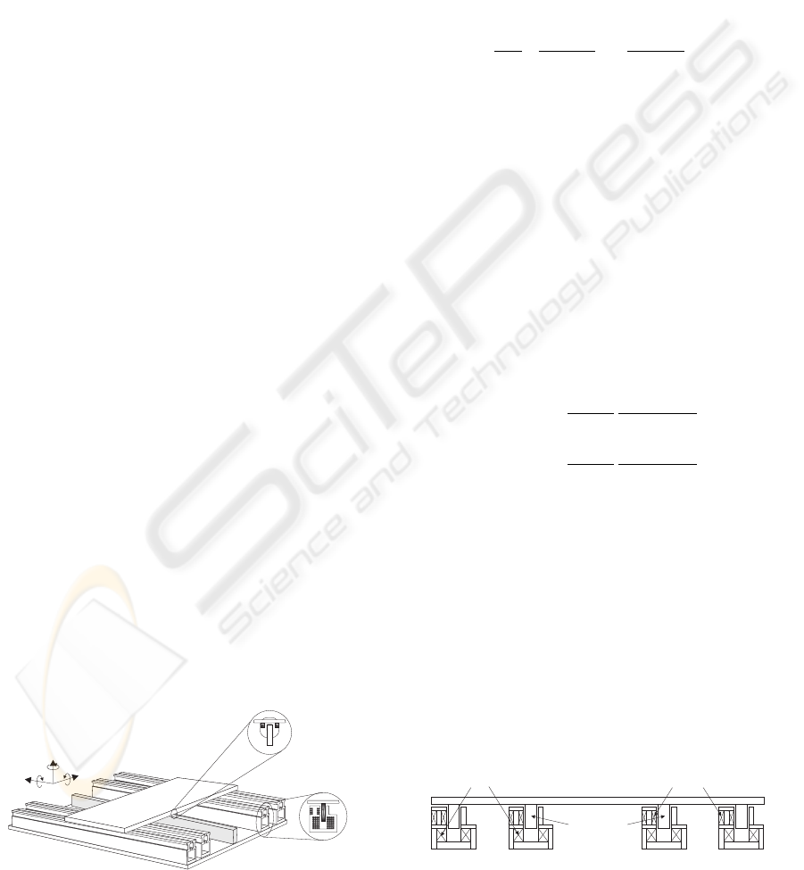
controlled in a future work. The overall system is
shown in Fig.1.
2.1 Maglev system
Basically, the maglev system proposed here is a multi-
input multi-output (MIMO) system. Here, the states
are the lateral and vertical displacement, x and z re-
spectively, and the three rotations θ, ψ and φ. The
outputs are x, θ, z, ψ and φ while the inputs are the
currents applied to coils into the levitation guiding
tracks. The dynamics of the maglev system can be
divided into a stable part and an unstable one. The
stable part consists of the dynamic of z, while the un-
stable part consists of the dynamics of x, θ, ψ and φ.
In order to control 3 DOFs in rotational displace-
ment and 2 DOFs in lateral displacement, i.e., a total
of 5 DOFs of the carrier separately, a four-track de-
sign, shown in Fig.2, is sufficient to supply such 5-
DOFs control. The guiding tracks together must pro-
vide a levitation force to counteract the carrier weight.
On the other hand, to provide a uniform magnetic
field along the guiding tracks, an oblong coil is nec-
essary.
Also, due to the nature of lateral instability of a re-
pulsive system, stabilizers are needed inside.The sta-
bilizers can control the lateral position of a levitat-
ing NdFeB magnet whereas the levitator can control
the vertical (up-down) position of a levitating NdFeB
magnet.
z
y
x
q
f
y
Carrier
Guidingtrack
PropulsionDevice
Figure 1: 3D view of maglev system
The four stabilizing coils are grouped into two sets:
inner guiding tracks and outer guiding tracks. Then,
the principle shown in Figs.3 and 4 to control the ro-
tation of the carrier about a vertical axis and its lateral
translation can be used.
In order to obtain the magnetic force in z and x
is necessary to analyze some magnetic formulas. Ac-
cording to Biot-Savart’s law and Ampere’s circuit law
(Nayef and Brussel, 1985) the magnetic flux density
in any point around an infinitely long current-carrying
straight wire at a point (x,z) can be obtained as
B =
µ
0
I
2π
−z
x
2
+ z
2
ˆ
i +
x
x
2
+ z
2
ˆ
k
(1)
where µ
0
is the permeability of free space, I is the in-
put current,
ˆ
i and
ˆ
k are the unit vector in the Cartesian
coordinate.
If we deal with a permanent magnet as a single di-
pole moment, the expression of the Lorentz force F
exerted on the permanent magnet by an external mag-
netic field B can be characterized by the following
vector equation
F = (u · ∇) B (2)
where u is the dipole moment of the permanent mag-
net. Assuming that the dipole lies in the z direction,
useful scalar equations of the force components can
be derived from (2) as
F
x
=
µ
0
Iu
z
2π
z
2
− x
2
(x
2
+ z
2
)
2
(3)
F
z
=
µ
0
Iu
z
π
−xz
(x
2
+ z
2
)
2
(4)
2.2 Nonlinear model
Consider a carrier represented by an uniform box-
shaped object with the center of mass coincident with
the center of geometry. The principle of linear mo-
mentum leads to the following equations:
F
x
= m¨x, F
z
= m¨z (5)
where F
x
and F
z
are the resultant forces acting on the
carrier along the x-axis and z-axis, respectively, and
m is the mass of the carrier.
carrier
TrackA TrackB TrackDTrackC
levitationcoils
stabilizingcoils
permanent
magnets
Figure 2: Front view of the maglev system
ICINCO 2005 - SIGNAL PROCESSING, SYSTEMS MODELING AND CONTROL
100
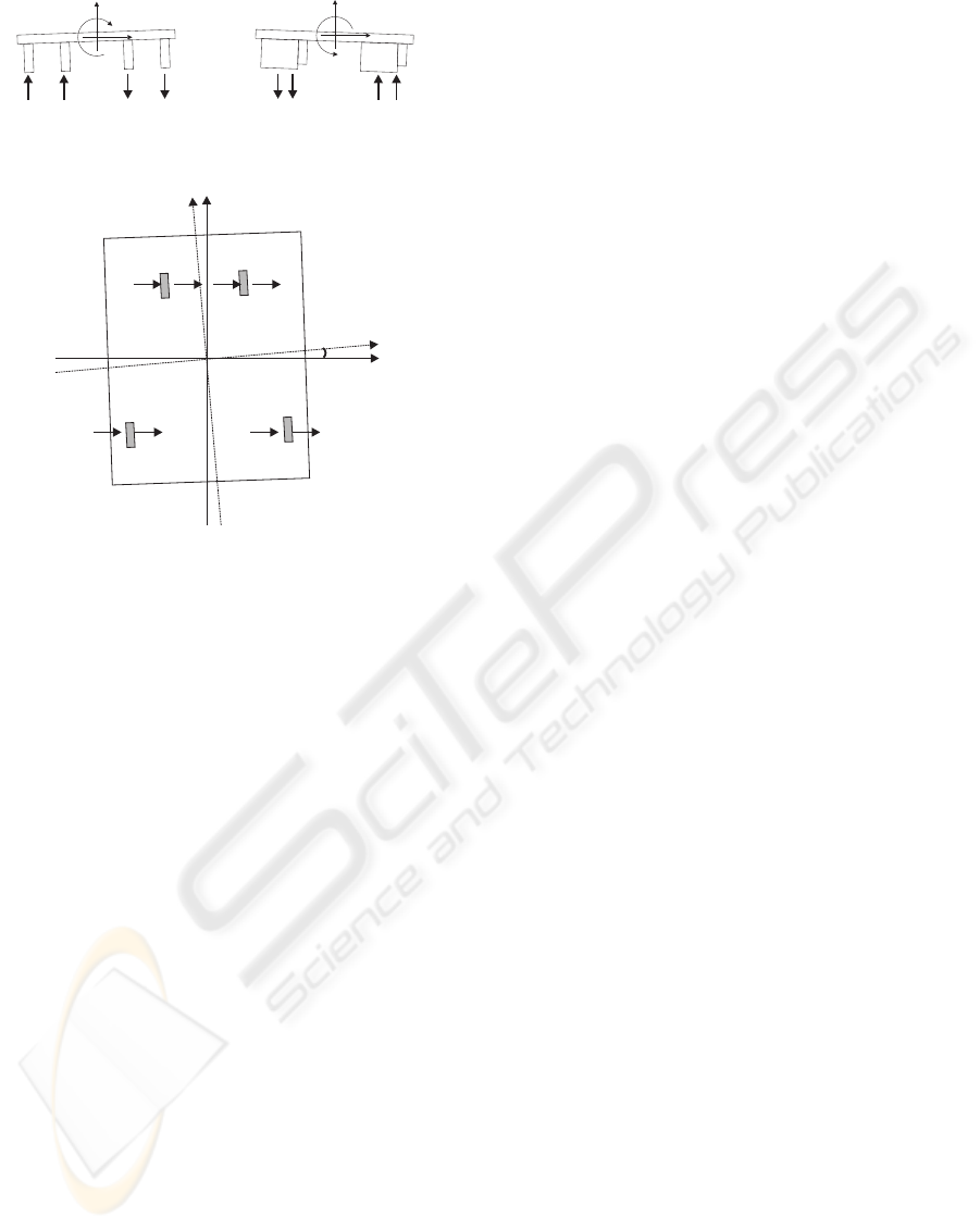
z
y
f
z
x
y
FZA FZB FZDFZC FZAFZBFZD FZC
Figure 3: Magnetic levitation forces
x
.y
_q
A B
C D
Fxad FxbdFxas Fxbs
Fxcd Fxcs Fxdd Fxds
Figure 4: Destabilizing and stabilizing forces
By the same token, the principle of angular mo-
mentum leads to torque equations for the rotational
coordinates
T
z
= J
z
θ, T
y
= J
y
ψ, T
x
= J
x
φ (6)
where T
z
,T
y
and T
x
are the external torques, J
z
, J
y
and J
x
are the principal moments of inertia and θ, ψ
and φ are the three angular rotation of the rigid body.
To understand the dynamics of the maglev system
it is necessary to describe an arbitrary orientation of
the carrier in space. This orientation can be obtained
using the Euler angular description yaw(θ)-roll(ψ)-
pitch(φ) given by the following rotation matrix
R =
"
cθcψ cθsψsφ − sθcφ
sθcφ sθsψsφ + cθcφ
−sψ cψsφ
cθsψcφ + sθsφ
sθsψcφ − cθsφ
cψcφ
#
(7)
where c and s represents cos and sin respectively.
The position of the levitation magnets on the carrier
are
A (−b
1
, a, 0) B (b
1
, a, 0)
C (−b
2
, −a, 0) D (b
2
, −a, 0)
where A, B, C and D denote the center position of
these magnets and a, b
1
and b
2
are known dimensions.
If one assumes small pitch, roll and yaw angle for the
carrier, in additional to x and z translation, the posi-
tion of the magnets on the carrier can be calculated
as
b
(x,y,z)a
=
"
−b
1
− aθ + x
a − b
1
θ
b
1
ψ + aφ + z
#
b
(x,y,z)b
=
"
b
1
− aθ + x
a + b
1
θ
−b
1
ψ + aφ + z
#
b
(x,y,z)c
=
"
−b
2
+ aθ + x
−a − b
2
θ
b
2
ψ − aφ + z
#
b
(x,y,z)d
=
"
b
2
+ aθ + x
−a + b
2
θ
−b
2
ψ − aφ + z
#
(8)
In similar form, the positions of the magnets into the
guiding tracks, shown in Fig.5, are obtained as
"
x
a,b
y
a,b
z
a,b
#
=
"
−aθ + d
l
ψ + x
a − d
l
φ
aφ + d
l
+ z
#
"
x
c,d
y
c,d
z
c,d
#
=
"
aθ + d
l
ψ + x
−a − d
l
φ
−aφ + d
l
+ z
#
(9)
Before formulating equations of motion, some nota-
tions on force and distances are explained in the fol-
lowing: the force subscript has two letters, the first
means the label of the magnet, and the second the
magnetic force type, d for destabilizing, s for stabi-
lizing and l for levitation, e.g. F
ad
is the destabilizing
force applied to the magnet A caused by the levita-
tion coil A . The position of the magnets, denoted by
b, has a subscript with two letters, the first means the
direction of the distance and the second the label of
the magnet, e.g. b
xa
is the distance in the x direction
from the carrier center to the center of the magnet A.
By substituting the positions of the levitation mag-
net (9) into the magnetic force equations (3) and (4)
one can get the forces exerted on each levitation mag-
net. Next, one can substitute these force equations
into the dynamics of the carrier, and then the equa-
MODELING AND CONTROLLER DESIGN OF A MAGNETIC LEVITATION SYSTEM WITH FIVE DEGREES OF
FREEDOM
101
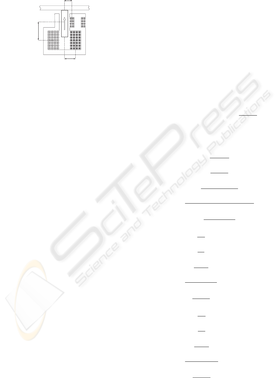
ds
dd
dl
Figure 5: Guiding track
tions of motion can be obtained as
m
t
¨x = F
ad
I
a
+ F
as
I
s1
+ F
bd
I
b
+ F
bs
I
s1
+F
cd
I
c
+ F
cs
I
s2
+ F
dd
I
d
+ F
ds
I
s2
J
z
¨
θ = −b
ya
F
ad
I
a
− b
ya
F
as
I
s1
− b
yb
F
bd
I
b
−b
yb
F
bs
I
s1
+ b
yc
F
cd
I
c
+ b
yc
F
cs
I
s2
+b
yd
F
dd
I
d
+ b
yd
F
ds
I
s2
m
t
¨z = F
al
I
a
+ F
bl
I
b
+ F
cl
I
c
+ F
dl
I
d
+F
p
− m
t
g
J
y
¨
ψ = b
xa
(F
al
I
a
− w
a
) − b
xb
(F
bl
I
b
− w
b
)
+b
xc
(F
cl
I
c
− w
c
) − b
xd
(F
dl
I
d
− w
d
)
−b
za
F
ad
I
a
− b
za
F
as
I
s1
− b
zb
F
bd
I
b
−b
zb
F
bs
I
s1
− b
zc
F
cd
I
c
− b
zc
F
cs
I
s2
−b
zd
F
dd
I
d
− b
zd
F
ds
I
s2
J
x
¨
φ = b
ya
(F
al
I
a
− w
a
) + b
yb
(F
bl
I
b
− w
b
)
−b
yc
(F
cl
I
c
− w
c
) − b
yd
(F
dl
I
d
− w
d
)
(10)
where g is the acceleration due to gravity, m
t
is the
mass of the carrier and load, J represents the mo-
ment of inertia of the carrier, w represents the weight
above each magnet, I
s1
is the current in the inner sta-
bilizer whereas I
s2
is the current in the outer stabi-
lizer. I
a
, I
b
, I
c
, I
d
represent the currents in the levita-
tors corresponding to the levitation magnets A, B, C
and D respectively. F
p
represents the damping force
produced by the levitation coils and can be modeled
as F
p
= −K
dam
˙z, where K
dam
is a positive constant.
3 CONTROLLER DESIGN
In this section , a control scheme is presented for the
levitation an stabilization dynamics of the magnetic
system described in section 2. The aim is to control
the height z while the lateral and rotational displace-
ments are tried to be kept near to zero. For doing this
a SOSM proposed in (Elmali and Olgac, 1992) is ap-
plied to the nonlinear model (10). For symplicity, the
currents in the levitation coils A and B are set to be
same, thus I
ab
= I
a
= I
b
. One also defines the state
vector ρ =
h
x ˙x θ
˙
θ z ˙z ψ
˙
ψ φ
˙
φ
i
T
together with the
input vector u = [I
ab
I
c
I
d
I
s1
I
s2
]
T
and the output
vector y = [x θ z ψ φ]
T
. The nonlinear model (10)
can then be rewritten in the state space form
˙ρ = f (ρ) + ∆f (ρ) +
5
X
i=1
[g
i
(ρ) + ∆g
i
(ρ)] u
i
y = h (ρ) (11)
where
f (ρ) = col
˙x, 0,
˙
θ, 0, ˙z,
−g −
K
dam
˙z
m
t
,
˙
ψ, 0,
˙
φ, 0
i
∆f (ρ) = col[0, 0, 0, 0, 0, ∆f
6
(ρ), 0, 0, 0, 0]
g
1
(ρ) =
0
F
ad
+F
bd
m
t
0
F
al
+F
bl
m
t
0
−b
ya
F
ad
−b
yb
F
bd
J
z
0
b
xa
F
al
−b
xb
F
bl
−b
za
F
ad
−b
zb
F
bd
J
y
0
b
ya
F
al
+b
yb
F
bl
J
x
g
2
(ρ) =
0
F
cd
m
t
0
F
cl
m
t
0
b
yc
F
cd
J
z
0
b
xc
F
cl
−b
zc
F
cd
J
y
0
−b
yc
F
cl
J
x
g
3
(ρ) =
0
F
dd
m
t
0
F
dl
m
t
0
b
yd
F
dd
J
z
0
b
xd
F
dl
−b
zd
F
dd
J
y
0
−b
yd
F
dl
J
x
ICINCO 2005 - SIGNAL PROCESSING, SYSTEMS MODELING AND CONTROL
102

g
4
(ρ) =
0
F
ae
+F
be
m
t
0
0
0
−b
ya
F
ae
−b
yb
F
be
J
z
0
−b
za
F
ae
−b
zb
F
be
J
y
0
0
g
5
(ρ) =
0
F
ce
+F
de
m
t
0
F
ce
+F
de
m
t
0
b
yc
F
ce
+b
yd
F
de
J
z
0
−b
zc
F
ce
−b
zd
F
de
J
y
0
0
∆g
j
(ρ) =
∆g
1j
(ρ)
.
.
.
∆g
10j
(ρ)
j = 1, . . . , 5
h (ρ) = [ρ
1
ρ
3
ρ
5
ρ
7
ρ
9
]
T
∆f (ρ) and ∆g
j
(ρ) represent modeling uncertainties
associated to the magnetic system. Equation (11) can
also be written in a more condensed form as
˙ρ = f (ρ) + ∆f (ρ) + [G (ρ) + ∆G (ρ)] u
y = h (ρ) (12)
where
G (ρ) = [g
1
(ρ) . . . g
5
(ρ)]
∆G (ρ) = [∆g
1
(ρ) . . . ∆g
5
(ρ)]
The goal is to make the output y (ρ) in system (12)
follow a desired trajectory y
d
(t). The control strat-
egy should be robust enough to handle the modeling
uncertainties ∆f and ∆G. The upper bounds of these
equations are assumed to be
|∆f
6
(ρ)| ≤ σ (ρ)
|∆g
ij
(ρ)| ≤ α
ij
(ρ) i = 1, . . . , 10
j = 1, . . . , 5 (13)
When the modeling uncertainties are not considered,
this is ∆f (ρ) = 0 and ∆G (ρ) = 0, one has the exact
model
˙ρ = f (ρ) + G (ρ) u
y = h (ρ) (14)
for which one can easily verify, in accordanace to
(Isidori, 1995) that it has a (vector) relative degree
[r
1
, r
2
, r
3
, r
4
, r
5
] = [2, 2, 2, 2, 2] at a point ρ
0
= 0. In
particular the decoupling matrix A (ρ) is given by
A (ρ) =
a
11
· · · a
15
.
.
.
.
.
.
.
.
.
a
51
· · · a
55
(15)
where
a
ij
= L
g
j
L
f
h
i
= g
(2i)j
(ρ) i, j = 1, . . . , 5
which is nonsingular at ρ = 0. One can also verify
that, for the uncertain system (12),
∆f (ρ) and
∆G (ρ) ∈ Ker
h
dh
i
, dL
f
h
i
, . . . , dL
r
i
−2
f
h
i
i
(16)
for i = 1, . . . , 5. This is, the so-called matching con-
dition is achieved. Thus the uncertainties ∆f and ∆G
do not appear in the time derivatives of y
i
of order
less than r
i
= 2 and the (vector) relative degree is
unchanged. Besides, since
P
5
i=1
r
i
= 10, system
(12) has no unobservable internal dynamics. Follow-
ing (Elmali and Olgac, 1992), a SOSM strategy that
allows to have reference output tracking despite the
presence of the uncertainties can be obtained by set-
ting
˙s
j
+ z
0
s
j
= ˙e
j
+ c
j1
e
j
+ c
j0
Z
e
j
j = 1, . . . , 5 (17)
where s
j
= ˙s
j
= 0 represents the jth sliding surface
and e
j
= y
j
− y
jd
is the jth tracking error, with y
jd
being the jth component of the desired output y
d
. The
constant real coefficients c
j0
and c
j1
are chosen in
such a way that the polynomial π
2
+ c
j1
π + c
j0
= 0
is Hurtwitz. z
0
is also a constant real coefficient.
By choosing a Lyapunov function candidate as
V
j
=
1
2
˙s
T
˙s + ω
2
n
s
T
s
for j = 1, . . . , 5 (18)
where s = [s
1
, . . . , s
5
]
T
and ω
n
is a real coefficient,
one has that, the Lyapunov stability criterion leads to
the condition
˙s
T
¨s + ω
2
n
s
≤ 0 (19)
which is known as the attractivity condition towards
s = ˙s = 0. By setting
¨s = −Ksgn ( ˙s) − ω
2
n
(20)
where K is a real positive number different from zero
and sgn ( ˙s) = [sgn ( ˙s
1
) , . . . , sgn ( ˙s
5
)]
T
, one can as-
sures the fulfillment of condition (19). From this last
MODELING AND CONTROLLER DESIGN OF A MAGNETIC LEVITATION SYSTEM WITH FIVE DEGREES OF
FREEDOM
103
equation and considering the exact model (14) one has
the sliding control u = u
s
given by
u
s
= −A
−1
(ρ)
h
F (ρ) + CE − y
(r)
d
− z
0
˙s
i
−A
−1
(ρ)
Ksgn ( ˙s) + ω
2
n
s
(21)
where
F (ρ) =
L
2
f
h
1
L
2
f
h
2
L
2
f
h
3
L
2
f
h
4
L
2
f
h
5
=
0
0
−g −
K
dam
m
t
ρ
6
0
0
CE =
c
10
e
1
+ c
11
˙e
1
.
.
.
c
50
e
5
+ c
51
˙e
5
y
r
d
= [¨y
d1
. . . ¨y
d5
]
T
For the uncertain system (12) (this is ∆f 6= 0 and
∆G 6= 0), when the sliding control u
s
is substituted
into (19), the attractivity condition takes the form
˙s
T
−K
I + ∆A (ρ) A
−1
(ρ)
sgn ( ˙s)
+∆A (ρ) A
−1
(ρ) (bv − F (ρ)) + ∆F (ρ)
< 0
(22)
where
∆A (ρ) =
L
∆g
j
L
f
h
1
.
.
.
L
∆g
j
L
f
h
5
j = 1, . . . , 5
∆F (ρ) =
L
∆f
L
f
h
1
L
∆f
L
f
h
2
L
∆f
L
f
h
3
L
∆f
L
f
h
4
L
∆f
L
f
h
5
=
0
0
∆f
6
0
0
bv = y
r
d
− CE + z
0
˙s − ω
2
n
s
One can notice that ˙s
T
sgn ( ˙s)≥k ˙sk, thus
−K ˙s
T
sgn ( ˙s)≤−K k ˙sk, and (22) can be reiter-
ated using vector norms obtaining
−K + K
∆AA
−1
sgn ( ˙s)
+
∆AA
−1
(bv − F )
+ k∆F k ≤ −µ (23)
where µ > 0. This last expression leads to the follow-
ing
K ≥
∆AA
−1
(bv − F )
+ k∆F k + µ
1 − k∆AA
−1
sgn ( ˙s)k
(24)
were it is assumed that
∆AA
−1
sgn ( ˙s)
< 1.
4 SIMULATION RESULTS
In this section, a series of simulation are proposed
for the maglev system using the SOSM controller de-
signed in the previous section. The simulation para-
meters are listed in table 1. The desired values for
all states are equal to zero, this means that the perma-
nent magnets are regulated at the center of the guid-
ing tracks whereas the carrier is located in the center
of the system.
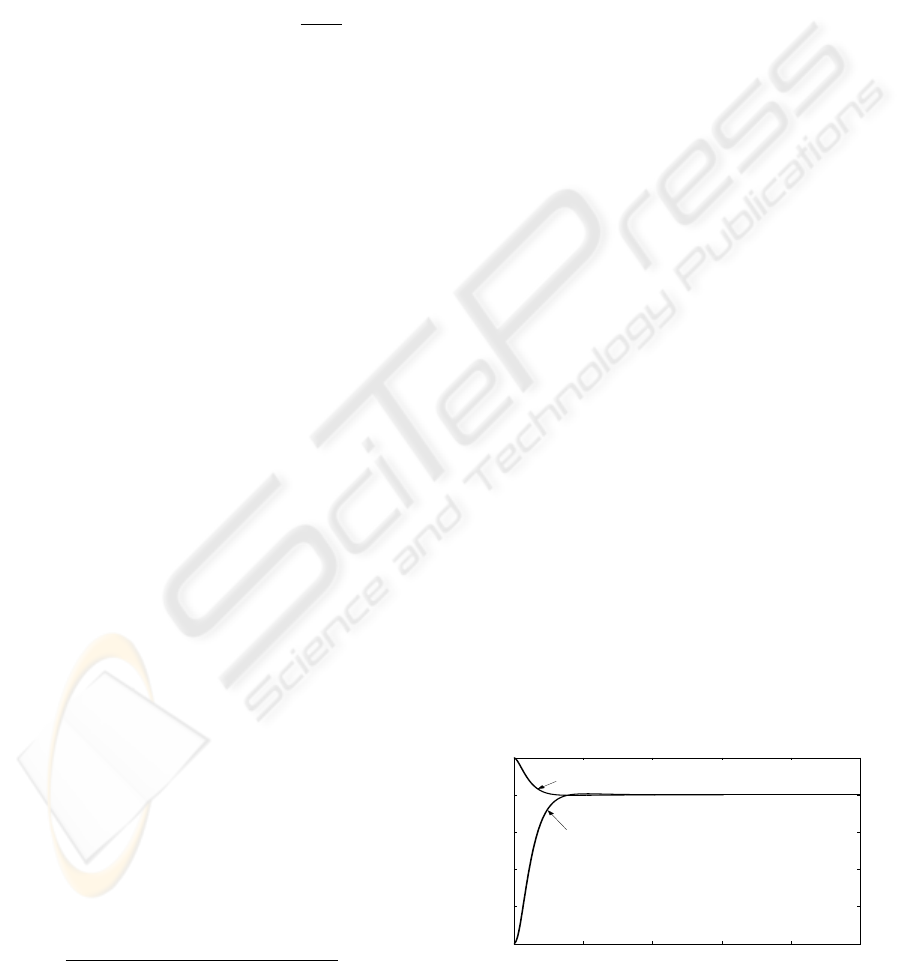
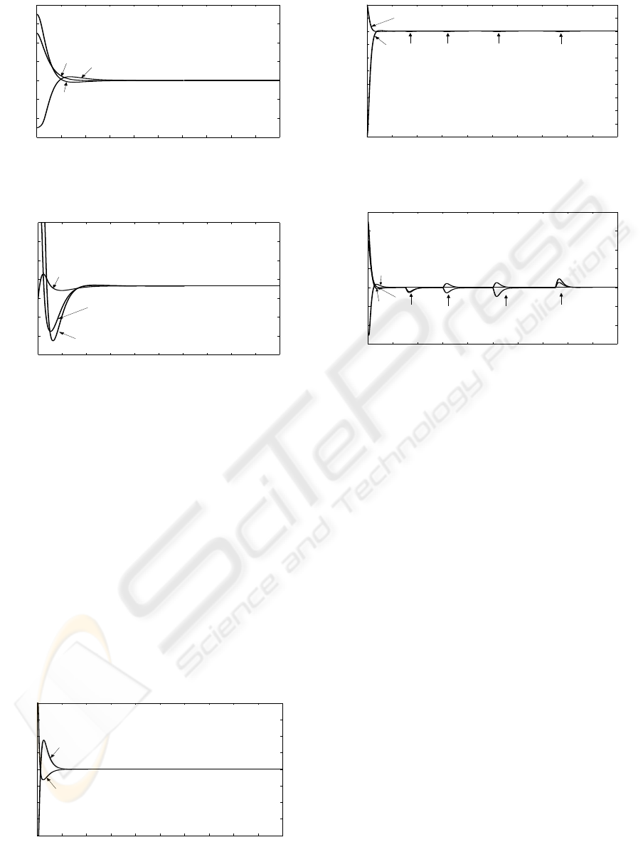
The first simulation was made with no load pertur-
bations and with the initial conditions x (0) = 2 mm,
θ (0) = 25 mrad, z (0) = −8 mm, ψ (0) =
35 mrad and φ (0) = −25 mrad. Figures 6 and 7
show that all the states converge to zero as t goes to
infinity. Figures 8 and 9 show the levitation and sta-
bilization control currents, respectively. In Fig.9 one
can notice that the stabilization control currents have
a zero value at steady state, this means that permanent
magnets are located at the center of the guiding tracks,
where the destabilizing forces are equal to zero.
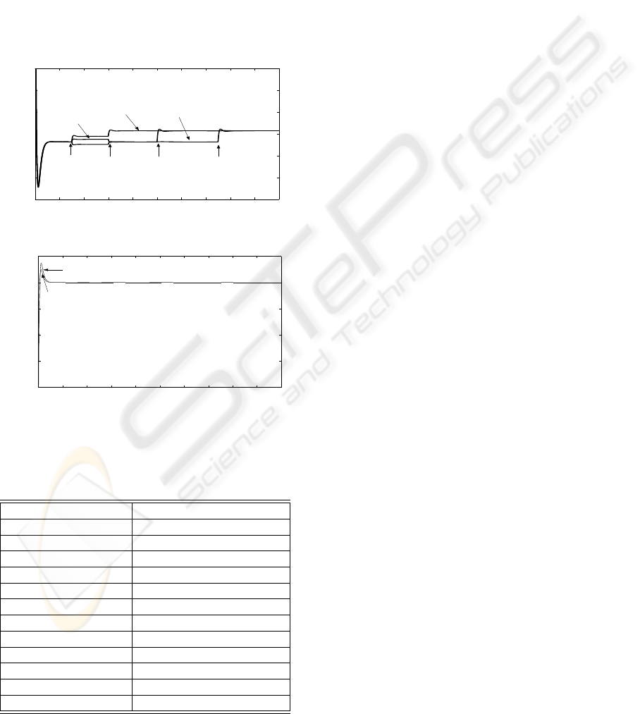
The second simulation tests the capability of load
disturbance rejection. The load disturbance is applied
on the carrier over each levitation magnet (see figures
3 and 4) after the carrier reaches a steady-state. Dis-
turbances of 0.25 Kg are introduced at 0.3s, 0.6 s, 1
s and 1.5 s. In this case, the initial conditions were
x (0) = 2 mm, θ (0) = 2.5 mrad, z (0) = −8 mm,
psi (0) = 3.5 mrad and φ (0) = −2.5 mrad. Figu-
res 10 and 11 show the response of the maglev system
when a load disturbance is applied on the carrier. One
can observe that all the states go to equilibrium points
when the load disturbance increases. Fig.12 shows
the changes in the levitation control currents due to
different load disturbances; one can observe the in-
crements or decrements in the current magnitude after
the load disturbance increases. Fig.13 shows that the
currents in both stabilizers do not present any change,
this is because the load does not affect the x transla-
tion and the θ rotation.
0 0.1 0.2 0.3 0.4 0.5
−8
−6
−4
−2
0
2
time (s)
distance (mm)
x
z
Figure 6: Carrier motion in x and z without load distur-
bances
ICINCO 2005 - SIGNAL PROCESSING, SYSTEMS MODELING AND CONTROL
104
0 0.05 0.1 0.15 0.2 0.25 0.3 0.35 0.4 0.45 0.5
−30
−20
−10
0
10
20
30
40
time (s)
rotation (mrad)
θ
ψ
φ
Figure 7: Carrier rotations θ, ψ and φ without load distur-
bances
0 0.05 0.1 0.15 0.2 0.25 0.3 0.35 0.4 0.45 0.5
−0.5
0
0.5
1
1.5
2
2.5
3
time (s)
current (amp)
I
ab
I
c
I
d
Figure 8: Levitation currents A, C and D without load dis-
turbances
5 CONCLUSIONS
In this paper a nonlinear mathematical model for a
maglev system has been derived. A repulsive ma-
glev system with four guiding tracks is adopted here.
There, the maglev system has been treated as a MIMO
system, and a SOSM controller for a nonlinear 5
DOFs maglev system has been designed here. From
the simulation results, the feasibility and effectiveness
of the designed controller have been clearly shown.
The desired performances of levitation and lateral and
rotational stabilization have been achieved. Future
work includes experimental laboratory tests.
0 0.1 0.2 0.3 0.4 0.5 0.6 0.7 0.8 0.9 1
−2
−1.5
−1
−0.5
0
0.5
1
1.5
2
time (s)
current (amp)
I
e1
I
e2
Figure 9: Stabilization currents 1 and 2 without load distur-
bances
0 0.2 0.4 0.6 0.8 1 1.2 1.4 1.6 1.8 2
−8
−7
−6
−5
−4
−3
−2
−1
0
1
2
time (s)
distance (mm)
x
z
L
1
L
2
L
3
L
4
Figure 10: The carrier motion with load disturbances
0 0.2 0.4 0.6 0.8 1 1.2 1.4 1.6 1.8 2
−3
−2
−1
0
1
2
3
4
time (s)
rotation (mrad)
θ
φ
ψ
L
1
L
2
L
3
L
4
Figure 11: Carrier rotations with load disturbances
REFERENCES
Bartolini, G., Ferrara, A., Pisano, A., and Usai, E. (2001).
On the convergence properties of a 2-sliding control
algorithm for non-linear uncertain systems. In Inter-
national Journal of Control, vol. 74, no.7, pp. 718-
731. Taylor Francis Ltd.
Castro-Linares, R., Glumineau, A., Laghraouche, S., and
Plestan, F. (2004). Higher order siding mode oberver-
based control. In in 2nd Symposium on System, Struc-
ture and Control, Oaxaca, Mexico, pp. 517-522.
Elmali, H. and Olgac, N. (1992). Robust output tracking
control of nonlinear mimo systems via sliding mode
technique. In Automatica, vol. 28, no. 1, pp. 145-151.
Pergamon Press plc.
Isidori, A. (1995). Nonlinear Control Systems. Springer
Verlag, New York, 3rd edition.
Jacobs, W. A. (2001). Magnetic launch assist-nasa’s vision
for the future. In IEEE Transactions on Magnetics,
vol. 37, no. 1, pp. 55-57.
Kaloust, J., Ham, C., Siehling, J., Jongekryg, E., and Han,
Q. (2004). Nonlinear robust control design for levi-
tation and propulsion of a maglev system. In in IEE
Proc. Control Theory Appl., vol. 151, no.4, pp. 460-
464. IEE.
Khamesse, M. B., Kato, N., Kamura, Y., and Nakamura, T.
(2002). Design and control of a microrobotic system
using magnetic levitation. In IEEE/ASME Transac-
tions on Mechatronics, vol. 7, no. 1, pp. 1-14. IEEE.
MODELING AND CONTROLLER DESIGN OF A MAGNETIC LEVITATION SYSTEM WITH FIVE DEGREES OF
FREEDOM
105
Kim, W.-J. and Trumper, D. L. (1998). High-precision mag-
netic levitation stage for photolithography. In Preci-
sion Engineering, vol. 22, no. 2, pp. 66-77. Elsevier
Science Inc.
Luguang, Y. (2002). Progress of high-speed maglev in
china. In IEEE Transactions on Applied Supercon-
ductivity, vol. 12, no. 1, pp. 944-947. IEEE.
Nayef, M. H. and Brussel, M. K. (1985). Electricity and
Magnetism. John Wiley and Sons, Inc., New York.
Suk, K. and Baek, Y. S. (2002). Contact-free moving-
magnet type of micropositioner with opimized spec-
ification. In IEEE Transactions on Magnetics, vol. 38,
pp. 1539-1548.
0 0.2 0.4 0.6 0.8 1 1.2 1.4 1.6 1.8 2
0
0.5
1
1.5
2
2.5
3
time (s)
current (amp)
I
ab
I
d
I
c
L
1
L
2
L
3
L
4
Figure 12: Behavior of the levitation A, C and D currents
0 0.2 0.4 0.6 0.8 1 1.2 1.4 1.6 1.8 2
−2
−1.5
−1
−0.5
0
0.5
time (s)
current (amp)
I
e1
I
e2
Figure 13: Behavior of the stabilization 1 and 2 currents
Table 1: System parameters
Mass m 1.0536 Kg
Carrier dimension 405 x 205 x 6 mm
NdFeB Size 13.91 x 31.62 x 25.4 mm
NdFeB Br 1.19 T
Turns of levitator 240 turns
Turns of stabilizer 120 turns
diameter of wire 0.71 mm
a, b
1
, b
2
70, 81, 175 mm
d
e
, d
d
, d
l
12, 15, 17 mm
c
10
, c
20
, c
30
, c
40
, c
50
2,2,1,2,2
c
11
, c
21
, c
31
, c
41
, c
51
50,40,40,50,50
K,K
dam
170, 27
ω
n
, z
0
75, 0.7
ICINCO 2005 - SIGNAL PROCESSING, SYSTEMS MODELING AND CONTROL
106
