
IMAGE BINARISATION USING THE EXTENDED KALMAN FILTER
Alexandra Bartolo, Tracey Cassar, Kenneth P. Camilleri
Department of Microelectronics
Simon G. Fabri
Department of Electrical Power and Control Engineering
Jonathan C. Borg
Department of Manufacturing Engineering
University of Malta
Keywords:
Feature Extraction, Image Processing, CAD.
Abstract:
Form design is frequently carried out through paper sketches of the designer’s mental model of an object.
To improve the time it takes from solution concept to production it would therefore be beneficial if paper-
based sketches can be automatically interpreted for importation into three-dimensional geometric computer
aided design (CAD) systems. This however requires image pre-processing before initiating the automated
interpretation of the drawing. This paper proposes a novel application of the Extended Kalman Filter to guide
the binarisation process, thus achieving suitable and automatic classification between image foreground and
background.
1 INTRODUCTION
Line drawing interpretation systems are used in en-
gineering design as an interface between engineer-
ing or architectural drawings and computer-aided de-
sign (CAD) tools (Ablameyko S. and Pridmore T.,
2000). Using similar principles, sketch recognition
systems are being developed since it is acknowledged
that designers can express their ideas more naturally
by means of sketches (Roth-Koch S., 2000). Recent
developments of such recognition systems have fo-
cused on online sketches obtained by means of PDAs
or tablet PCs. Since such systems are online, the in-
terpretation system has additional information about
the drawing, for example, pen position and velocity.
However, these systems lack the portability and flex-
ibility of paper (Farrugia P. et al., 2004). In order
to achieve this flexibility, the images must be pre-
processed, such that line data may be extracted from
the static image. Binarisation is one such process,
which compensates for the noise introduced by the
digitizing system. This work proposes the use of the
Extended Kalman Filter (EKF) to guide the binarisa-
tion of images as a step towards the automation of the
sketch recognition process which provides the neces-
sary data to control rapid prototyping and manufac-
turing equipment. The proposed method improves
the binarisation of poor quality images, whilst reduc-
ing the complexity of the threshold selection process.
This paper is divided as follows: Section 2 gives a
brief review of binarisation techniques, Section 3 in-
troduces the EKF and illustrates how this filter may
be used to identify a suitable threshold for binarisa-
tion. This is followed by the results in Section 4 and
conclusions in Section 5.
2 BINARISATION TECHNIQUES
Binarisation is the process by which grey levels
within an image are classified as either foreground or
background (Ablameyko S. and Pridmore T., 2000).
The selection of a suitable binarisation technique is
dependent on the type and quality of the images be-
ing used (Bulen S. and Mehmet S., 2004). Since
the sketched line drawing interpretation system that is
being developed is expected to process images from
the field, it will typically process poor quality im-
ages, digitized using low-resolution devices, such as a
camera-phone. This requires a more detailed and lo-
cal analysis of the pixel distributions in order to select
a suitable threshold for pixel classification. This sec-
tion describes five established binarisation techniques
originally proposed for line drawings and text images.
160
Bartolo A., Cassar T., P. Camilleri K., G. Fabri S. and C. Borg J. (2005).
IMAGE BINARISATION USING THE EXTENDED KALMAN FILTER.
In Proceedings of the Second International Conference on Informatics in Control, Automation and Robotics - Robotics and Automation, pages 160-167
DOI: 10.5220/0001182101600167
Copyright
c
SciTePress

Palumbo and Guliano (Yang Y. and Yan H., 2000)
use a fixed 9 × 9 window to evaluate the class of each
pixel within the image. The pixel value is determined
according to the five 3 × 3 local pixels within the
9 × 9 window centered on the pixel in consideration.
An initial threshold is used to determine the pixels
which definitely belong to the background whilst the
remaining pixels are classified using a different label
assignment rule requiring the specification of three
additional user defined parameters. Determining the
values of these thresholds is not straightforward since
they cannot be deduced from the image properties.
Niblack’s algorithm (Bulen S. and Mehmet S.,
2004) evaluates a threshold for each pixel within the
image according to the mean and standard deviation
of the pixels in a predetermined window W centered
at the pixel in consideration. The pixel class is deter-
mined as follows:
w(x, y) →
w
f
,p(x, y) <T(x, y)
w
b
,p(x, y) ≥ T (x, y)
(1)
where T (x, y)=µ(x, y)+k × σ(x, y), µ(x, y) is
the mean grey level of the pixels within the window,
σ(x, y) is the standard deviation of these pixels and k
is a user defined parameter. Niblack’s algorithm re-
quires two user defined parameters. The window size
determines the number of pixels from which the mean
µ(x, y) and standard deviation σ(x, y) are evaluated.
Thus, the window size should reflect the quality of the
image background, on which prior knowledge is un-
available. The value of k is used to adjust the amount
of print object boundary that is taken as part of the
foreground, and is therefore dependent on the quality
of the drawn line which is also an unknown quantity.
Eikvil’s method (Trier O. D. and Jain A. K., 2000)
is based on Otsu’s thresholding technique (Gonzalez
R. and Woods R. E., 2002), and makes use of two con-
centric windows L and S. The pixels within the larger
window L are temporarily classified into two classes
by Otsu’s threshold. The mean of these two clusters is
evaluated and their difference is compared to a para-
meter k which determines whether there there is suffi-
cient contrast between the two clusters. This indicates
the effectiveness of Otsu’s threshold on the selected
region. Thus, if the difference between the two means
is larger than k, the pixels within the smaller window
are thresholded according to Otsu’s threshold. Other-
wise, the pixels are assigned to the class whose label
is closest to the mean grey level within the smaller
window S. This method requires the specification of
three user defined parameters, of which S and L de-
fine window sizes, whilst k determines the threshold-
ing method applied to the smaller window. The size of
the smaller window S may be set to 3 which defines
the smallest window centered on a pixel. However,
the remaining parameters must be specified according
to the particular image properties.
Kamel and Zhao’s logical adaptive tech-
nique (Kamel M. and Zhao A., 1993) compares
the grey level of the pixel in consideration with
eight local averages in a pixel neighborhood of size
(2SW +1)
× (2SW +1)where SW represents
the stroke width of the line drawing. A comparison
operator is derived from these averages and is used
to determine the class of the pixel in consideration.
The algorithm requires two user defined parameters,
namely the stroke width SW and an initial threshold
T which is used to evaluate the required comparison
operator. Yang and Yan (Yang Y. and Yan H., 2000)
proposed a method by which the two parameters
SW and T are calculated adaptively. However,
the adaptive evaluation of the parameter T requires
another parameter α. Yang and Yan (Yang Y. and Yan
H., 2000) specify a range of values of α for which
suitable values of T may be obtained.
Brensen’s method (Bulen S. and Mehmet S., 2004)
may either classify a single pixel or a group of pix-
els simultaneously according to the contrast present
within a selected window. The window’s contrast is
defined as C(x, y)=Z
max
− Z
min
, where Z
max
and Z
min
are the maximum and minimum grey levels
within the window. If this contrast is smaller than a
predefined value k, the pixels within the window be-
long to the same class, and the entire window may be
assigned to a single class. However, if the contrast C
is sufficiently large, then the pixels within that win-
dow belong to two different classes. Since the win-
dow has high contrast, a simple threshold based on
the average gray level may be used to classify the pix-
els within this window. Thus, the threshold T is de-
fined as T (x, y)=
1
2
× (Z
max
+ Z
min
). This method
requires the specification of parameter k which may
be evaluated adaptively using the method proposed
in (Bartolo A. et al., 2004)
2.1 Drawbacks
Although the above methods may yield results of con-
siderably good quality, the classification processes re-
quires that a classifying criterion is evaluated for each
pixel in the image. Furthermore, these algorithms re-
quire the specification of some parameter, such as a
window size in order to evaluate the threshold. Al-
though suggested values are specified for some algo-
rithms, better results are obtained after fine-tuning the
parameter to the characteristics of the image under
test. Thus the performance of these methods is sus-
ceptible to image conditions. Methods for the adap-
tive evaluation for Brensen’s and Kamel & Zhao’s
methods have been proposed, but these require con-
siderable computational times, which slow down the
product prototyping process. In this paper, we attempt
to overcome these problems by modelling the sketch
as a trajectory being tracked in time.
IMAGE BINARISATION USING THE EXTENDED KALMAN FILTER
161

3 LINE TRACKING
A sketched drawing may be considered as a number
of lines which interact at junctions or corners to
create two-dimensional shapes. These lines may be
considered as distinct entities, which can be described
independently by some mathematical model. In this
paper, two mathematical models which describe the
position of a point on a line and its intensity are used
to enable line tracking. Each line stroke is modelled
as a trajectory propagating with a velocity v along a
line subtending an angle θ with the horizontal axis,
thus the position of the trajectory at a time instant
k +1is given by Equation (2), where x
1
and x
2
are
the vertical and horizontal coordinates on a plane.
x
1
(k +1)
x
2
(k +1)
=
x
1
(k)
x
2
(k)
+ v ×
sin θ
cos θ
(2)
Given a static, offline image, the velocity of propaga-
tion is irrelevant and may be assumed to be unity, thus
making the (x
1
,x
2
) coordinates of the line dependent
only on the direction θ. The bilinear interpolation
relationship given by Equation (3) (Gonzalez R.
and Woods R. E., 2002), can be used to describe the
intensity of a pixel in terms of its (x
1
,x
2
) coordinates,
z(k)=Ax
1
(k)+Bx
2
(k)+Cx
1
(k)x
2
(k)+D (3)
where A, B, C and D are interpolation coefficients
derived from the four neighbors of a pixel in the image
with coordinates (x
1
,x
2
).
In this way, each stroke in a given drawing may
be considered as a process modelled by Equation (2).
From the original image, measurements of pixel in-
tensities, given by Equation (3), can be obtained. By
considering the (x
1
,x
2
) coordinates of each line as
the states of a dynamic system and the intensity val-
ues to be measurements obtained from noisy sensors,
Kalman filter theory (Maybeck P. S. , 1982) may be
used to estimate the system states and hence the coor-
dinates of points on each line.
Since the relation between pixel intensity and pixel
position, given by Equation (3), is not linear, the
Extended Kalman Filter (EKF) was adopted. The
EKF linearizes the state estimation around the cur-
rent estimate by using the partial derivatives of the
process and measurement functions to compute esti-
mates even when non-linearities are present. How-
ever, stability of the EKF assumes that the process is
linear around the current state (Maybeck P. S. , 1982).
3.1 The Extended Kalman Filter
In general, the EKF addresses the problem of estimat-
ing the state x of a discrete-time process modelled by
nonlinear state-space equations of the general form:
x(k +1) = f (k, u(k), x(k)) + w(k) (4)
z(k)=h(k, x(k)) + v(k) (5)
where w represents the model noise and v the mea-
surement noise, which are zero-mean, Gaussian noise
sequences of covariance Q and R respectively, u is
a known input, z is a measured output and f and h
are general non-linear functions. In our line sketching
application, the line generator model given by Equa-
tion (2) is cast into the state space form of Equation
4 to give Equation (6). Similarly, Equation (3) which
represents the intensity model, is cast into the state
space form of Equation (5) to give Equation (7).
x(k +1) = x(k)+ θ(k)+w(k) (6)
z(k)=h(k, x(k)) + v(k) (7)
where the state vector
x ≡
x
11
,x
12
, ··· ,x
n1
,x
n2
T
represents pen positions on n line strokes in the im-
age,
θ(k) ≡
sin(θ
1
), cos(θ
1
), ··· , sin(θ
n
), cos(θ
n
)
T
represents the orientation of the lines. The intensity
of the trajectories at time k, is given by z, which may
be written as:
z
1
(k)=A
1
x
11
(k)+B
1
x
12
(k)+
C
1
x
11
(k)x
12
(k)+D
1
+ v
1
(k)
z
2
(k)=A
2
x
21
(k)+B
2
x
22
(k)+
C
2
x
21
(k)x
22
(k)+D
2
+ v
2
(k)
.
.
.
z
n
(k)=A
n
x
n1
(k)+B
n
x
n2
(k)+
C
n
x
n1
(k)x
n2
(k)+D
n
+ v
n
(k)
where A
i
, B
i
, C
i
and D
i
are known constants ob-
tained from the bilinear interpolation, given by Equa-
tion (3).
Comparison between Equations (4) and (6) gives
f (k, u(k), x(k)) = x(k)+θ(k), and h(k, x(k)) is
given by Equation (3). Process noise w(k) models
any deviations from the ideal line stroke, and mea-
surement noise v(k) corresponds to noise affecting
the intensity measurements of the image.
Based on the state space model given by Equa-
tions (6) and (7), the EKF algorithm is used to find an
estimate ˆx(k|k) to the actual state x(k), based upon
intensity measurements z(k) as follows (Maybeck P.
S. , 1982):
The Kalman Gain is defined as:
K(k)=
P(k|k − 1)∇
T
h(ˆx(k|k−1))
∇
h(ˆx(k|k−1))
P(k|k − 1)∇
T
h(ˆx(k|k−1))
+ R
(8)
ICINCO 2005 - ROBOTICS AND AUTOMATION
162
where
∇
h(x)
≡
⎛
⎜
⎝
∂h
1
∂x
11
∂h
1
∂x
12
··· 00
.
.
.
.
.
.
.
.
.
.
.
.
.
.
.
00···
∂h
n
∂x
n1
∂h
n
∂x
n2
⎞
⎟
⎠
represents the rate of change in intensity in the verti-
cal and horizontal directions for each line stroke.
The state estimate is obtained by:
ˆx(k|k)=ˆx(k|k − 1)+
K(k)
z(k) − h(k, ˆx(k|k − 1))
(9)
where z(k) represents the true intensity measured
from the image and h(k, ˆx(k|k−1)) is given by Equa-
tion (3) evaluated at x(k)=ˆx(k|k − 1). The error
Covariance P(k|k) is given by:
P(k|k)=[I − K(k)∇
h(ˆx(k|k−1))
]P(k|k − 1) (10)
where the covariance prediction is:
P(k +1|k)=J
f (ˆx(k|k))
P (k|k)J
T
f (ˆx(k|k))
+ Q (11)
where J
f (x)
is the Jacobian matrix
∂f
i
∂x
j
, which in
this case is equivalent to the identity matrix from
Equation (6). The state estimate prediction at time
k +1is:
ˆx(k +1|k)=f (k, u(k), ˆx(k|k)) (12)
The EKF Equations (8) to (12) will recursively
compute the state estimate ˆx(k|k) for each iterate k,
given initial estimates ˆx(0|−1) = x
0
and initial co-
variance P(0|−1) = P
0
which represents the ini-
tial covariance of the error, reflecting the initial un-
certainty of the estimates.
3.2 Application to binarisation
The EKF equations described above, give the possi-
bility of locating points on a number of lines that form
part of the drawn object or objects in an image. In this
way, the EKF helps to discriminate between the image
foreground and background by selecting those pixels
which are located on lines and are therefore part of the
image foreground. The intensity of the pixels along
the tracked trajectory provides information about the
grey level intensities of the pixels forming part of the
line drawing. The mean grey level intensity µ
t
, and
standard deviation σ
t
of the tracked pixels can there-
fore be used to approximate the grey-level intensity of
the sketched object, and hence guide the binarisation
process. Since line pixels are darker than the back-
ground, the image pixels are classified by comparison
to a threshold T = µ
t
+ n × σ
t
,where n is a con-
stant which defines the tolerance to grey-level varia-
tions along the tracked line. Pixels whose intensities
are less than T may be classified as foreground line
pixels whilst the remaining pixels may be classified
as background pixels.
0 50 100 150 200 250 300 350
−0.15
−0.1
−0.05
0
0.05
0.1
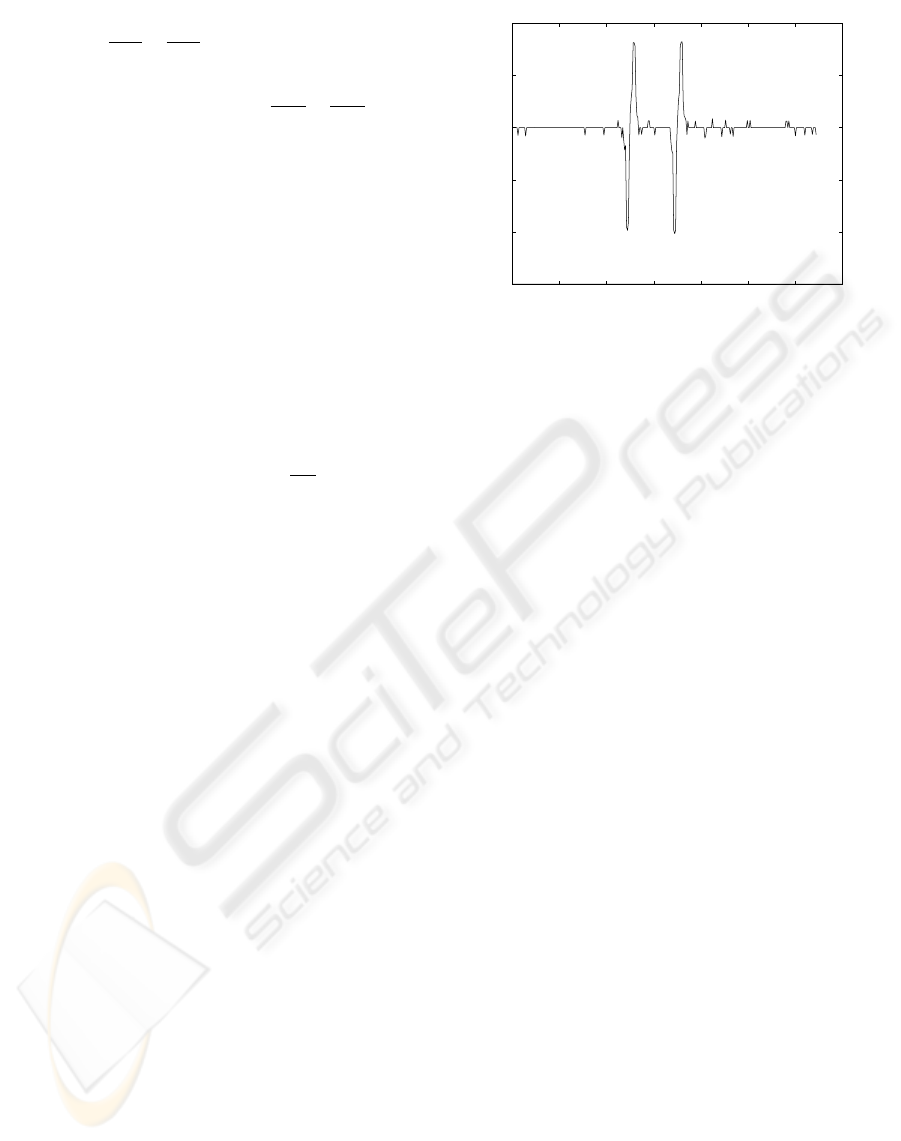
Figure 1: The derivative of a horizontal row in an image.
Each positive - negative peak indicates the presence of a
line.
3.3 Implementation of the EKF
The implementation of the EKF requires suitable
starting points to initialize the line tracking process.
The position of the lines in a static image are un-
known, however, it may be assumed that part of the
image will be located towards the center of the im-
age. Thus, two scans along the horizontal and vertical
centerlines of the image are performed. The deriva-
tive of the grey level intensities of pixels lying along
this line is considered. The presence of a line is indi-
cated by a negative and positive peak along the track-
ing direction, which correspond to the two edges of
the line stroke as shown in Figure 1. Suitable start-
ing points may be taken at the midpoints of two such
peaks. Since a horizontal and a vertical scan are car-
ried out, the EKF can be initialized with at least two
starting points.
Since sketches are not necessarily built from
straight lines, but may have curves or lines that ex-
hibit a change in orientation, the sketched strokes are
modelled as piece-wise linear segments. This implies
that the line stroke may be built from a number of
short straight line segments which may be represented
by the state space model shown in Equation (6), thus
requiring the evaluation of the line orientation θ(k) at
each iteration k. This may be obtained by using Sobel
edge response (Gonzalez R. and Woods R. E., 2002),
which gives the magnitude response and the orienta-
tion of the pixels within the image. For edge pixels,
the magnitude response is highest and the pixel orien-
tation corresponds to the orientation of the line. Thus,
for each state ˆx, the closest edge pixel pair are located
and their orientation is used as an approximation for
the line direction θ(k).
The state estimates given by Equations (9) require
the evaluation of the intensity of the image at instant
IMAGE BINARISATION USING THE EXTENDED KALMAN FILTER
163

k. This may be obtained by searching for the darkest
gray level within a distance of one unit from the cur-
rent pixel position in the direction of θ +∆θ where
the ∆θ term is used to allow for deviations in the line
direction. Since the line strokes are expected to be
smooth, any line deviation from θ is accommodated
by seeking the darkest pixels in the cardinal directions
that enclose θ.
Since the EKF assumes that the model used is lin-
ear around the current state, large deviations from the
line stroke would cause the filter to diverge. For this
reason, it is required to terminate the tracking before
the filter diverges. An indication that the filter is di-
verging may be obtained by comparing the gray level
intensity of the tracked point with the grey level in-
tensity of background pixels. A measure of the back-
ground intensity may be obtained by taking the mean
gray-level m
s
of a sample of pixels located at a dis-
tance d perpendicular to the line direction, where d
should be greater than the stroke width of the sketched
lines. A point located on an image line will have a
gray level m
p
which is less than the mean gray level
m
s
of the sample pixels. Thus, divergence is indi-
cated when the mean gray level m
s
of the sampled
pixels is less than or equal to the gray level inten-
sity m
p
of the tracked point thus indicating that the
point is no longer on the sketched line and has moved
to a background region. This criterion also detects
when the tracking point arrives at the end of a line and
is therefore also used as a criterion to terminate the
tracking process once the end of the line is reached.
The image digitization process introduces some de-
gree of noise to the image such that adjacent pixels
will have variations in their gray level intensity even
though they belong to the same class. This will in-
troduce errors in the evaluation of the EKF starting
points since the derivative of an image row or column
will also reflect these intensity variations. For this rea-
son the image is low pass filtered using a 3 × 3 mean
filter (Gonzalez R. and Woods R. E., 2002). This will
reduce the effect of the gray level variations in adja-
cent pixels making the transition between image class
more prominent in the row and column derivatives.
4 TESTING AND RESULTS
The proposed algorithm was tested under various con-
ditions and compared to the performance of the other
established methods discussed in Section 2. This sec-
tion shows the results obtained for a number of sam-
ple grey level images, whose gray levels are in the
range [0 256]. The visual results obtained by Kamel
and Zhao’s method are also shown in order to allow
a visual comparison. Kamel and Zhao’s method has
been chosen as this has the lowest number of user de-
Figure 2: Illustrating the tracking paths generated by the
EKF. White line segments indicate the tracked path, whilst
the darker lines indicate the image line strokes. This exam-
ple shows the tracking of 11 segments.
fined parameters and thus offers the highest degree of
automation.
The ability of the EKF to track multiple lines was
first tested with images having a low noise compo-
nent as shown in Figure 2. This shows an example
where the EKF tracks eleven segments, correspond-
ing to seven starting points detected from a horizontal
scan and four segments detected from a vertical scan
of the image.
The algorithm was then tested under varying de-
grees of measurement noise. This was introduced by
adding zero-mean Gaussian noise to the image. Fig-
ure 3 illustrates a ground truth image consisting of
4913 foreground pixels and 81651 background pix-
els. The corresponding noisy image is shown in Fig-
ure 3(b). The noise added has a standard-deviation
of 36 grey-levels, which corresponds to a signal-to-
noise ratio (SNR) of 12.8dB. The results obtained by
the EKF algorithm and Kamel and Zhao’s algorithm
are shown in Figure 3(c) and 3(d) respectively. Fur-
ther results are given in Table 1. These show that
the results obtained by the EKF algorithm have lower
Table 1: Comparison of percentage pixel error of the EKF
algorithm and Kamel and Zhao’s algroithm under different
noise conditions for the image shown in Figure 3(a). f→b
indicates the percentage foreground misclassification and
b→f the percentage background misclassification.
% pixel error
EKF Kamel & Zhao
SNR(dB) f → b b → f f → b b → f
18.08 7.1 0.53 17.9 0.79
16.20 14 0.07 26 1.19
14.54 12.2 0.18 35.8 1.59
12.79 2.9 0.97 44.7 1.9
ICINCO 2005 - ROBOTICS AND AUTOMATION
164

Table 2: Number of lines tracked and the sample points
considered, given as a percentage of the total number of
pixels in the image for the images shown in Figure 4
Image Lines Tracked % Points Tracked
4(a) 7 0.24
4(b) 4 0.27
4(c) 7 0.36
Table 3: Comparison of computational times with the al-
gorithms discussed in Section 2 for the images shown in
Figure 4
Computational Time (s)
Image 4(a) 4(b) 4(c)
EKF 57.3 26.3 55.9
Eikvil 75.2 73.7 75.4
Brensen 160 139.5 137.9
Kamel 78.6 78.8 70.9
Niblack 30.7 30.5 39.8
Palumbo 12.5 9.7 13
foreground misclassifications and background mis-
classifications in comparison to the results obtained
by Kamel and Zhao’s method. This indicates that the
EKF algorithm gives a better performance than that of
Kamel and Zhao under noisy conditions.
Figure 4 illustrates three images used to test the
algorithm. These include multiple lines and curves,
which illustrate that the line tracking process may
effectively track such images. The number of lines
tracked and the sample points taken is tabulated in Ta-
ble 2.
This indicates that the thresholding decision is
based on a small number of pixels, which however,
correspond to pixels directly related to the image fore-
ground. The binary result obtained for these images
is illustrated in Figure 5. The results obtained may
be compared with those illustrated in Figure 6, which
are obtained by using Kamel and Zhao’s algorithm
after manually determining the most suitable values
for α. These results show that the proposed EKF al-
gorithm gives results whose quality is comparable to
those given by other binarisation thechniques. Fur-
thermore, Table 3 shows that the proposed binarisa-
tion process requires lower computational times than
Brensen’s and Kamel & Zhao’s methods, for which
adaptive parameter evaluation was applied. Although
Niblack’s, and Palombo and Guiliano’s methods show
lower computational times, this does not include the
time required to find suitable parameters for each im-
age, because, these are not adaptive methods.
The algorithm was also tested on images captured
by a cameraphone at a resolution of 96 dpi. A sam-
ple of these images is shown in Figure 7 where Fig-
ure 7(a) shows an image drawn on plain white paper,
Figure 7(c) shows an image drawn on textured tissue
paper whilst Figures 7(e) and 7(g) show images drawn
on graph paper. Note that the cameraphone captures
the light reflections on the image such that the result-
ing digital images display variable gray-level inten-
sities along the background. This is particularly ev-
ident in the image corners, where the gray-level in-
tensity of the background is comparable to that of the
foreground. The performance of the EKF algorithm is
comparable to that of the algorithms discussed in Sec-
tion 2 but require smaller computational times. Fig-
ure 7 shows how the algorithm correctly identifies the
foreground pixels. Of particular importance is the
distinction made between the image foreground and
the background grid in Figures 7(e) and 7(g), which
allows the extraction of the object from interfering
backgrounds. Some misclassification of the back-
ground pixels in the corner regions occurs for images
in Figure 7(f) and 7(h). This is due to the fact that the
image is being thresholded with a global threshold.
The images shown in Figure 7(f) and 7(h) have some
foreground pixels with a relatively high gray level in-
tensity, resulting in a higher valued threshold, which
will classify the darker background regions as fore-
ground.
5 CONCLUSION
The proposed EKF binarization method has been
shown to yield good quality results that are compa-
rable to those obtained by existing methods. Further
work is being carried out in order to apply the algo-
rithm to local image regions, resulting in a number of
local thresholds rather than a single global threshold.
This will reduce the effect of global thresholding, thus
further improving the results obtained.
The proposed method offers a higher degree of au-
tomation than the other binarization techniques dis-
cussed since no user defined parameters are required.
This helps to improve the rapid prototyping process
of the sketched line drawing, which is the main, long
term objective of this work.
ACKNOWLEDGEMENTS
This work has been mainly supported by Grant 73604
of the University of Malta.
IMAGE BINARISATION USING THE EXTENDED KALMAN FILTER
165
(a) (b) (c) (d)
Figure 3: Illustrating the performace of the EKF binarisation under noise. Figure (a) shows a ground truth image and Figure
(b) shows the corresponding image with added Gaussian noise resulting in an SNR of 15.5dB. Figures (c) and (d) show the
binary result obtained by the EKF method and Kamel & Zhao’s method respectively.
(a) (b) (c)
Figure 4: Sample test images. Images (a) and (b) illustrate image having a homogenous background with dynamic ranges of
160 and 80 respectively, whilst Image (c) is an example of an image having background artefacts.
(a) (b) (c)
Figure 5: Results given by the EKF binarisation for images shown in Figure 4.
(a) (b) (c)
Figure 6: Results given by Kamel & Zhao’s method for images shown in Figure 4, with α equal to 0.4, 0.2, 0.1 respectively.
ICINCO 2005 - ROBOTICS AND AUTOMATION
166
100 200 300 400 500 600
50
100
150
200
250
300
350
400
450
100 200 300 400 500 600
50
100
150
200
250
300
350
400
450
100 200 300 400 500 600
50
100
150
200
250
300
350
400
450
100 200 300 400 500 600
50
100
150
200
250
300
350
400
450
(c) (d)
100 200 300 400 500 600
50
100
150
200
250
300
350
400
450
100 200 300 400 500 600
50
100
150
200
250
300
350
400
450
100 200 300 400 500 600
50
100
150
200
250
300
350
400
450
100 200 300 400 500 600
50
100
150
200
250
300
350
400
450
(g) (h)
Figure 7: Results obtained by the EKF binarisation algorithm for a set of real test data captured with a cameraphone using a
resolution of 96 dpi. Figures a), c), e) and g) show the original images whilst Figures b), d), e) and h) show the binary result.
REFERENCES
Ablameyko S. and Pridmore T. (2000). Machine Interpre-
tation of Line Drawing Images. Springer-Verlag.
Bartolo A., Camilleri K., Borg J., and Farrugia P. (2004).
Adaptation of Brensen’s Thresholding Algorithm for
Sketched Line Drawings. Eurographics Workshop on
Sketch-Based Interfaces and Modeling, pages 81–90.
Bulen S. and Mehmet S. (2004). Image Thresholding Tech-
niques - A Survey over Categories. Journal of Elec-
tronic Imaging, 13:146–165.
Farrugia P., Borg J., Camilleri K., Spiteri C., and Bartolo
A. (2004). A Cameraphone-Based Approach for the
Generation of 3D Models from Paper Sketches. Eu-
rographics Workshop on Sketch-Based Interfaces and
Modeling, pages 34–42.
Gonzalez R. and Woods R. E. (2002). Digital Image
Processing. Prentice Hall.
Kamel M. and Zhao A. (1993). Extraction of Binary Char-
acter/Graphics from Grey Level Document Images.
CVGIP: Graphical Models and Image Processing,
55(3):203–217.
Maybeck P. S. (1982). Stochastic Models, Estimation and
Control, Volume 2. Academic Press.
Roth-Koch S. (2000). Generating CAD Models from
Sketches. Proceedings of the IFIP WG5.2 Geomet-
ric Modeling: Fundamentals and Applications, pages
207–219.
Trier O. D. and Jain A. K. (2000). Goal directed evaluation
of binarisation methods. Workshop on Perfromance
versus Methodology in Computer Vision, 17(3):209–
217.
Yang Y. and Yan H. (2000). An Adaptive Logical Method
for Binarisation of Degraded Document Images. Jour-
nal of the Pattern Recognition Society, 33:787–807.
IMAGE BINARISATION USING THE EXTENDED KALMAN FILTER
167
