
IMPROVEMENT ON THE POLE-PLACEMENT CONTROL
SCHEME BY USING GENERALIZED SAMPLED-DATA HOLD
FUNCTIONS
David J. Donaire, Rafael Bárcena, Koldo Basterretxea
Department of Electronics and Telecommunications, University of the Basque Country, La casilla 3, Bilbao, Spain
Keywords: sampled-data systems; GSHF; pole-placement control.
Abstract: This paper studies the benefits the use of GSHF can afford to the pole-placement control scheme. The
GSHF
makes possible to locate the zeros of the discretized plant arbitrarily in the Z plane. This property can
be taken advantage of to improve the performance of the pole-placement control. In this article a new design
method is suggested and a simulations-based application example is carried out. In the application example
the improvements this method involves with respect to the classical design method are noticed.
1 INTRODUCTION
Usually, most sampled data control systems use the
Zero Order Hold (ZOH). However, some authors
((Kabamba, 1987) (Bai and Dasgupta, 1990) (Er and
Anderson, 1994) (Yan et al., 1994) (Rossi and
Miller, 1999) (Barcena abd De la Sen, 2003)) have
proved that using hold patterns which differ from the
zero order extrapolation, that the ZOH carries out,
can improve the discrete performance of the hybrid
system.
The GSHF (Generalized Sampled-data Hold
Fu
nction), device which has been widely studied
(Kabamba, 1987) (Bai and Dasgupta, 1990) (Er and
Anderson, 1994) (Yan et al., 1994), has a generic
hold function which can be tuned to obtain some
advantages. For example, (Kabamba, 1987) proves
that the zeros of the discretized plant can be placed
arbitrary in the Z plane by tuning the hold function
of the GSHF.
Several hybrid control schemes are based on the
cancellation
of the zeros of the discretized plant with
the controller poles. The pole-zero cancellation
cannot be done if there is any unstable zero in the
discretized plant, because it would make the system
internally unstable (Jury, 1956). This cancellation
would not be advisable either if there is any
insufficiently damped zero, since the cancellation of
this zero could cause intersample ripple (Clarke,
1984). It is always possible, by using the GSHF, to
stabilize the zeros of the discretized plant, when are
unstable, or to increase the stability degree of the
critically damped ones, in order to make possible a
safe cancellation. Therefore, this device makes
possible the use of mentioned control schemes.
On the other hand, it is well known (Kuo, 1992) that
th
e relative location of the zeros from the poles
influences in the system response. Therefore, the
GSHF can be used to place the zeros of the
discretized plant in more favourable locations from
the viewpoint of the control strategy and, in that
way, to improve the performance achieved with the
ZOH.
Although the mentioned advantages, both
conce
rning the discrete performance of the hybrid
system, some authors ((Feuer and Goodwin, 1994)
(Freudenberg et al., 1995) (Freudenberg et al.,
1997)) have proved that the use of the GSHF can
cause intersample difficulties which do no appear
when the ZOH is used. Nevertheless, this happens in
designs in which the intersample ripple these devices
can cause has not been taken into account. However,
when this possibility is taken into account by the
design method, it is possible to get somewhat degree
of improvement in the discrete performance of the
hybrid systems, without incurring in a too large
deterioration of the intersample performance. An
example of this appears in (Hjalmarsson and
Braslavsky, 1999).
Using the GSHF carries another adverse
effect: its
static hold function requires that the control signal
varies even during the steady-state. This can cause
the actuator fatigue and accelerate its wear. In (Chan,
2002) it is suggested an alternative to the static hold
pattern of the GSHF. The device suggested in that
92
J. Donaire D., Bárcena R. and Basterretxea K. (2005).
IMPROVEMENT ON THE POLE-PLACEMENT CONTROL SCHEME BY USING GENERALIZED SAMPLED-DATA HOLD FUNCTIONS.
In Proceedings of the Second International Conference on Informatics in Control, Automation and Robotics - Signal Processing, Systems Modeling and
Control, pages 92-98
DOI: 10.5220/0001181900920098
Copyright
c
SciTePress
paper converges asymptotically toward a ZOH input
pattern as the controlled system response tends to the
steady-state step response. This eliminates the
unceasing magnitude changes and the ripple the
control signal suffers during the steady-state step
response when the GSHF is employed. The analysis
of this device, variable GSHF from now on, and the
benefits its use can afford to the pole-placement
control will be the objectives of this paper.
This paper is organized in the following manner. In
section 2 the most important characteristics of the
variable GSHF are described and the pole-placement
control scheme structure is commented. In the
section 3 a new design method for this controller is
suggested. This design methodology takes into
account the variable GSHF properties so that the
benefits that this hold device can afford are taken
advantage of. In this way the pole-placement control
scheme performance is improved. In section 4 a
simulations-based application example is carried out
and the outcomes are compared with the obtained
ones by the classical design method. To finish, the
conclusions are drawn in the section 5.
2 PRELIMINARIES
2.1 Variable GSHF (Chan, 2002)
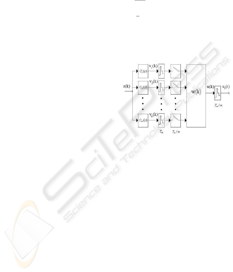
The variable GSHF contains m discrete filters which
process the incoming discrete signal with the sample
time T
m
. A MISO discrete filter of m inputs which
works with a sampling time of T
m
/m processes the
output signals of these m filters. The output signal of
this filter is rebuilt with a ZOH which works at the
same sampling rate. The Fig. 1 shows the structure of
the variable GSHF.
The variable GSHF divides the sampling time T
m
in
m subintervals and in each one of these subintervals
the hold function is kept constant. The amplitude
associated to each one subinterval depends on the
state of the MISO filter variable GSHF contains.
Therefore, the gains of each one subinterval may
vary from a sampling time to another. For that reason
we call it variable GSHF.
Using a variable GSHF with m=2 and a suitable
selection of the parameters of the discrete filters it is
possible to locate the zeros of any strictly proper
transfer function of arbitrary order which no contains
zeros, arbitrarily in the Z plane (Chan, 2002) (Chan,
1998). This is the case that we will study in this
paper.
The v
1
(z),...,v
m
(z)
filters are introduced to produce the
redundancy in the discrete control signal necessary
for zero placement. These filters are defined by (1)
where c
l
(z) and d(z) are polynomial of the same
degree. The MISO filter is defined by equation
system (2) where s
l
, with l=1,2,...,m, and p are
scalars.
()
() () , 1,2,...,
()
l
l
cz
vz rz l m
dz
==
(1)
1
1
1
() ()
2
() () ()
(0) 0
m
ll
l
m
l
l
wk pwk svk
uk wk v k
w
=
=
⎧
⎛⎞
+= +
⎪
⎜⎟
⎝⎠
⎪
⎪
⎪
=+
⎨
⎪
⎪
=
⎪
⎪
⎩
∑
∑
(2)
Figure 1: Variable GSHF
If the process to be controlled, discretized by the
ZOH contained in the GSHF, has the following
discrete-time
(1) () ()
() ()
dd
d
x
kAxkBu
yk Cxk
+= +
⎧
⎨
=
⎩
k
(3)
then, the state space representation of the system
composed of MISO filter and the discrete system
represented by (3) has the discrete time
representation described by the system (4).
1
(1) () ()
() ( 0)()
m
ll
l
d
zk Fzk Gv k
yk C zk
=
⎧
+= +
⎪
⎨
⎪
=
⎩
∑
(4)
where
()
()
()
x
k
zk
wk
⎛
=
⎜
⎝⎠
⎞
⎟
⎟
]
lm
∈
(5)
2
0
m
dd
AB
F
p
⎛⎞
=
⎜
⎝⎠
(6)
[
1
1
, 1,...,
0
i
m
d
dd
l
l
i
B
AB
G
s
p
−
=
⎛⎞
⎛⎞
=
⎜⎟
⎜⎟
⎝⎠
⎝⎠
∑
(7)
In the equation system (2) it is noticed that, when the
MISO settles, the signal which is reconstructed by
IMPROVEMENT ON THE POLE-PLACEMENT CONTROL SCHEME BY USING GENERALIZED SAMPLED-DATA
HOLD FUNCTIONS
93
the ZOH at each multiple of T
m
/m begin to update
only a time per sampling period. Therefore, the
variable GSHF behaves as a GSHF during transient
response and as a ZOH in the steady state. This
eliminates the unceasing changes of magnitude and
achieves to reduce the ripple that the static hold
pattern of the GSHF produces.
Using two subintervals (m=2), the assignment of the
discrete transfer function numerator is obtained
resolving the following diophantine equation:
11 2 2
1
() () () () () () ()
m
ll
l
g
zc z g zc z g zc z numz
=
=+ =
∑
(8)
where c
l
(z) are the numerator polynomial of the m
discrete filters which precede the MISO filter, num(z)
is the polynomial required as numerator of the
discretized plant transfer function and g
l
(z) is the
polynomial of the numerator of each one of the m
discrete systems obtained when the equation system
(4) is particularized to a concrete value of l.
It is important to point out that the implementation of
the variable GSHF involves no additional hardware
since the discrete filters are implemented in the
computer and, therefore, the only hardware needed to
implement this device is a ZOH.
2.2 Control scheme
In this paper the improvement the use of GSHF can
contribute to the pole-placement discrete control,
which is vastly studied in (Aström and Wittenmark,
1990), is analyzed.
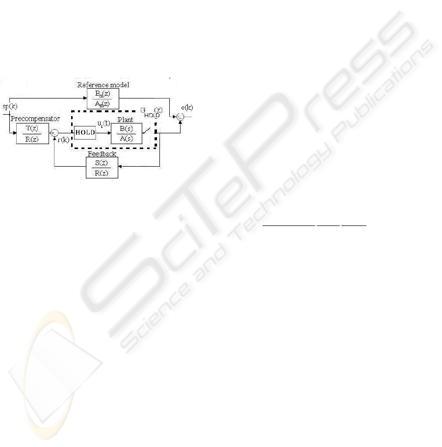
In this control scheme, which structure is represented
in Fig. 2, the polynomial R(z), S(z) and T(z) of the
discrete filters of the feedback loop and
precompensator are calculated to match the
behaviour of the closed-loop with the reference
model. This is carried out by solving the following
equations
0
0
() () () ()
() () ()() () ()
m
m
TzBz B zA z
A
zRz BzSz A zA z
=
+=
(9)
where A
0
(z) is a polynomial introduced to ensure the
solvability of the second equation of (9). The
discretized plant zeros are transmitted to the
reference model unless they are cancelled with the
controller poles. It is important to point out that only
stable zeros can be cancelled. For this reason the B(z)
polynomial is factorized into the following
polynomials: B
+
(z) and B
-
(z). Where B
+
contains the
stable zeros of the discretized plant the designer
wants to cancel and B
-
(z) contains the unstable zeros
and the stable zeros the designer decides to transmit
to the reference model. The zeros of the B
-
(z) are
necessarily roots of the numerator of the reference
model and, therefore, when B
-
(z) contains any zero,
the reference model cannot be chosen totally freely.
For this reason the polynomial B
m
(z) is factorized in
the following way
() () ' ()
m
Bz BzB z
−
=
m
(10)
where B’
m
(z) is the polynomial contained in B
m
that
can be chosen freely. In other respect, the polynomial
B
+
(z) is cancelled with the controller poles and
therefore the roots of B
+
(z) must be roots of the
polynomial R(z)
Figure 2: Reference model control scheme
() '()RBzRz
+
=
(11)
Using (10) and (11) in (9) the equations obtained are
0
0
() ' () ()
() '() ()() () ()
m
m
Tz B zA z
A
zR z B zSz A zA z
−
=
+=
(12)
By solving the equations (12) the discretized plant
behaviour is matched with the reference model
described by the equation (13).
0
0
'() () () ()
()
() ()
()
m
M
m
BzBzAzBz
Gz
Az Az
Bz
−+
+
=
(13)
3 DESIGN METHOD
This paper accomplishes the analysis of the
improvements that the GSHF can contribute to pole
placement control scheme. In this control scheme, the
first step is to locate the poles of the reference model
in terms of the required behaviour. Then, two
possibilities exist. It is possible to cancel the zeros
with controller poles or to transmit them to the
reference model. Is well known (Kuo, 1992) that the
relative position of the zeros from the poles
influences on the closed loop performance. In a
generic manner, to be able to relocate the zeros of the
closed loop anywhere in the Z plane supposes an
advantage. However, it is not always possible, since,
if the zeros of the plant are unstable or not
sufficiently damped, it is not advisable to cancel
them. Therefore, when the ZOH is the device used
for the reconstruction and the discrete transfer
function has this kind of zeros, we are forced to
transmit them to the reference model.
ICINCO 2005 - SIGNAL PROCESSING, SYSTEMS MODELING AND CONTROL
94
The variable GSHF, however, allows us to relocate
the zeros arbitrarily in the Z plane. Therefore, this
device permits to avoid these problems. Besides, two
possibilities exist.
The first method lies in using the variable GSHF to
locate the zero of the discretized transfer function of
the plant in the position where the reference model
has its zero. This allows achieving the model
matching without carrying out a cancellation.
The second way to match the closed-loop discrete
behaviour with the reference model using the GSHF
lies in positioning the zero of the discretized plant
transfer function in a place where the discrete zeros
are suitable to be cancelled without incurring in
intersample ripple. If the zero is located in a place
with this characteristic, then it is possible to cancel
this with the controller and to place the zero of the
system in the prescribed position.
4 APPLICATION EXAMPLE
In this section it is carried out a comparative study
between the performance attained in pole-placement
scheme by the ZOH and the attained one by a
variable GSHF, tuned as is described in section 3.
Both methods are applied for accurate positioning of
a computer hard disk read/write head. The model of
the read/write head used (Franklin et al., 1992) is
described by de following differential equation
() () () ()
i
It Ct Kt Kit
θθθ
++ =
(14)
where
I
is the inertia of the head assembly, C is the
viscous damping coefficient of the bearings, K is the
return spring constant, K
i
, is the motor torque
constant, i(t) is the input current and
θ
(t) is the
angular position of the head. With the parameters
suggested in (Franklin et al., 1992) (I=0.01 Kgm
2
,
C=0.004 Nm/rad, K=10Nm/rad y K
i
=0.005Nm/A)
the transfer function that describes the dynamic of
the plant is
2
5
()
0.4 1000
Gs
ss
=
++
(15)
To discretize a process, a usual agreement suggests
choosing the sampling time 20 times higher than the
continuous plant bandwidth (Kuo, 1992). To
accomplish with this agreement the sampling time is
fixed to 0.006 s. Pole-placement controller is the
scheme used in this section. The discrete behaviour
that is wished to transmit to the plant is described by
the following transfer function:
(
)
2
0.30417 0.4
()
1.2 0.3825
M
z
Gz
zz
−
=
−+
(16)
When the control objective is reached, the equivalent
damping coefficient of the closed-loop system is
about 0.89. This reference model has been chosen to
obtain the closed-loop system with the minimal
settling time. This selection is carried out due to the
fact that the settling time is one of the more
important specifications that the step response of a
hard disk needs to improve since the read/write
operation cannot start until the read/write head of the
hard disk places correctly in the position the
reference signal requires.
However, if the ZOH is used the obtained discrete
transfer function is
(
)
5
2
8.9659 10 0.9992
()
1.962 0.9976
ZOH
z
Gz
zz
−
⋅+
=
−+
(17)
This transfer function has its zero located almost on
the unit circle and it is not advisable to cancel this by
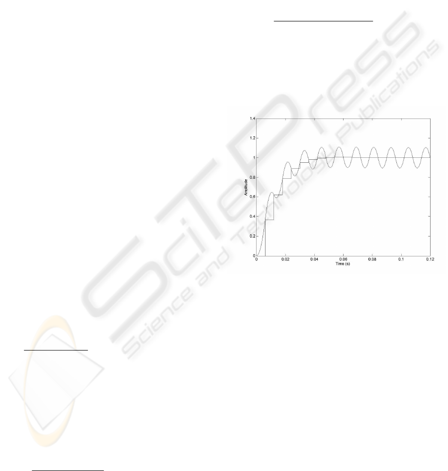
the controller. Fig. 3 shows the obtained result when
necessary cancellation to catch up with the discrete
reference model is carried out.
Figure 3: Unit-step response of the compensated system
by using ZOH device when discrete controller cancels the
discretization zero
.
Hence, it is necessary to transmit the zero of the
process to the reference model. When the zero is
transmitted to the reference model the system has the
step response shown in Fig. 4.
However, using GSHF it is possible to move the zero
from the place that it presents when ZOH is used. On
the one hand it is possible to use the GSHF to locate
the zero of the discrete transfer function of the plant
in the position where the reference model has its
zero. This allows achieving the model matching
without carrying out a cancellation. The variable
GSHF parameters used to locate the discretization
zero in z=0.4 are p=0, s
1
=1, s
2
=0.5, c
1
(z)=-13.8528z
- 1.1708, c
2
(z) = 18.3565z + 2.3416 and d(z)=z. In
Fig. 5 is depicted the step response of the system
when the related design method is achieved.
As is shown in Fig. 5 with the use of GSHF the
matching with the reference model (16) is attained
IMPROVEMENT ON THE POLE-PLACEMENT CONTROL SCHEME BY USING GENERALIZED SAMPLED-DATA
HOLD FUNCTIONS
95
without incurring in the generation of the intersample
ripple that the system was having when in the control
scheme the reconstruction device employed was the
ZOH (compare with Fig. 3). Comparing Fig. 4 and
Fig. 5 it is noticed that to be able to fit the model
reference model (16) when the GSHF is used
supposes an improvement: No one of both responses
present overshoot, but while the system which
employs ZOH settles in 0.52 s. the system that uses
GSHF needs only 0.41 s.. This supposes an
improvement of 21% in the settling time.
On the other hand, if the zero is located with the
GSHF at z=-0.2 (p=0, s
1
=1, s
2
=0.5, c
1
(z)=-4.6707z –
0.3344, c
2
(z) = 6.6713z + 0.6687 and d(z)=z) and
then is cancelled with a controller pole, the step
response of the closed loop is almost the same to the
obtained one in the case where the zero was directly
located in z=0.4.
The control signals of the three designs are depicted
in Fig. 6, Fig. 7 and Fig.8. In that figures it is noticed
that the reduction of the settling time is obtained at
expense of amplification of the control signal. The
amplification of the control signal is quite big, and
therefore, it is important to decide, depending on the
application, if the improvement obtained justifies the
amplification the control signal suffers respect the
ZOH case, or not. It is important to notice that in this
paper only two subintevals (m=2) are taken into
account and may be possible, with the use of more
subintervals, to reduce the control signal amplitude
during the transient response. However, if the
number of subintervals used is very high the ZOH
contained in the GSHF is forced to work at high rate.
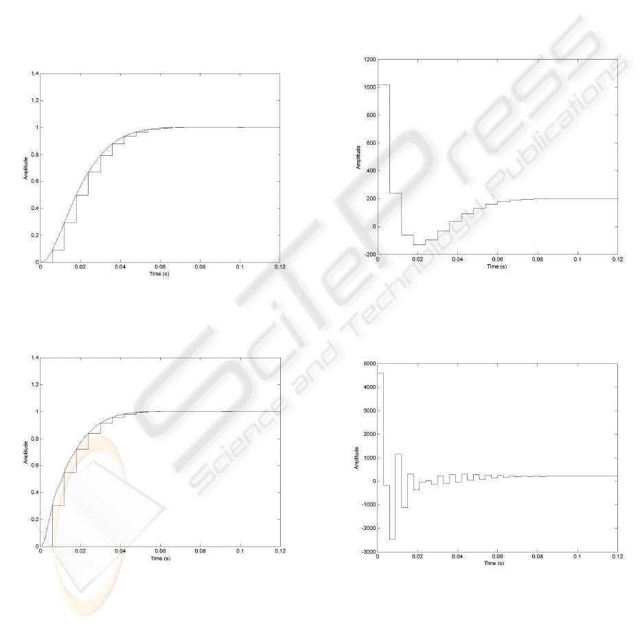
Figure 6: Control signal when the discrete plant zero is
transmitted to the reference model and ZOH is used.
Figure 4: Unit-step response of compensated system by
using ZOH device, when discrete plant zero is transmitted
to reference model.
Figure 7: Control signal of the design that uses the GSHF
to locate the zero in z=0.4 and this zero is transmitted the
discrete controller.
Figure 5: Unit-step response of compensated system by
using GSHF device to locate the zero in z=0.4 and this is
transmitted to reference model.
ICINCO 2005 - SIGNAL PROCESSING, SYSTEMS MODELING AND CONTROL
96
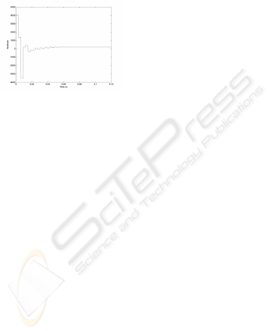
Figure 8: Control signal of the design that uses the GSHF
to locate the zero in z=-0.2 and this zero is cancelled by
the discrete controller.
5 CONCLUSION
In this paper, it has been noticed by means of an
application example that the variable GSHF can
improve the performance of the pole-placement
control scheme. The variable GSHF allowed us to
place the discretization zero of a second order
continuous plant in more beneficial location from the
viewpoint of the control strategy, improving in that
way the performance of the closed loop.
On the one hand, when the ZOH discretization zero
is sufficiently damped, it is possible to cancel it with
one of the controller poles and to locate the closed-
loop zero in the place where the reference model has
its zero. In such situations, the ZOH discretization
zero does not impose limitations to the attainable
performance and, therefore, the possibility of
relocating it that GSHF provides does not suppose
any advantage. On the other hand, when the ZOH
discretization zero is unstable or poorly damped,
which often happens when the sampling time used is
small enough (Aström et al., 1984), it is not advisable
to cancel it and, therefore, the performance that can
be attained by the classical design method is limited
given that the designer is forced to transmit such a
zero to the reference model in order to avoid
intersample ripple. This is the case studied in this
paper and it has been noticed that it is possible to
match the closed-loop discrete behaviour to the
reference model by the variable GSHF, without
generating intersample ripple.
From the carried out study it is concluded that the
GSHF ability to move the zeros can be used to
improve the transient response of a pole-placement
control. It has been also noticed that this
improvement is obtained at expense of the
amplification of the control signal during transient
state. It is important to point out that in this study it
has been used a variable GSHF with two subintervals
and it may be possible to reduce the control
amplitude by using more subintervals.
During the study, the possible deterioration of the
sensitivity functions, both discrete and hybrid ones,
have not been taken into account. That is one of the
possible drawbacks that the use of the GSHF can
generate (Freudenberg et al., 1997) and future
investigations on this device should integrate the
analysis of such functions.
REFERENCES
Kabamba, P. T., “Control of linear systems using
generalized sampled-data hold functions” IEEE Trans.
Automatic Control, Vol. AC-32, No. 9, pp.772-783
(1987)
Bai, E.-W., Dasgupta S., “A note on generalized hold
functions”, Systems & Control Letters, Vol. 14, pp.
363-368 (1990)
Er, M. J., Anderson B. D. O., “Discrete-time loop transfer
recovery via generalized sampled-data hold functions
based compensator”, Int. J. Robust Nonlinear Control,
Vol. 4, pp. 741-756 (1994)
Yan W.-Y., Anderson, B. D. O., Bitmead, R. R., “On the
gain margin improvement using dynamic
compensation based on generalized sampled data hold
functions”, IEEE Trans. Automatic Control, Vol. 39,
No. 11, (1994)
Rossi, M., Miller, D. E, “Gain/phase margin improvement
using static generalized sampled-data hold functions”,
Systems & Control Letters, Vol. 37, pp. 163-172
(1999)
Barcena, R., De la Sen, M., “On the sufficiently small
sampling period for the convenient tuning of
fractional-order hold circuits”, IEE Proc.-Control
Theory Appl., Vol. 150, No. 2 (2003)
Jury, E. I. “Hidden oscillations in sampled-data control
systems”, Trans. AIEE, 75, 391, (1956)
Clarke, D. W., “Self-tuning control of non minimum-
phase systems”, Automatica, 20, (5), pp. 501-517
(1984)
Kuo, B. C., (1992) Digital control systems, Saunders
College, 2
nd
edn
Feuer , A., Goodwin G.C., “Generalized hold functions-
Frequency domain analysis of robustness, sensitivity
and intersample difficulties”, IEEE Trans. Automatic
Control, Vol. 39, No. 5, pp.1042-1047 (1994)
Freudenberg, J., Middleton, R., Braslavsky, J., “Inherent
design limitations for linear sampled-data feedback
IMPROVEMENT ON THE POLE-PLACEMENT CONTROL SCHEME BY USING GENERALIZED SAMPLED-DATA
HOLD FUNCTIONS
97

systems”, Int. J. Control, Vol. 61, pp. 1387-1421
(1995)
Freudenberg, J., Middleton, R., Braslavsky, J.,
“Robustness of zero-shifting via generalized sampled-
data hold functions”, IEEE Trans. Automatic Control,
Vol. 42, No. 12, (1997)
Hjalmarsson, H., Braslavsky, J.H., “Tuning of controllers
and generalized hold functions in sampled-data
systems using iterative feedback tuning”, In Proc. of
the IFAC 14th World Congress, Beijing, China,
(1999)
Chan, J.-H. H., “Stabilization of discrete system zeros: An
improved design”, Int. J. Control, Vol. 75, No. 10, pp.
759-765 (2002)
Chan, J.-H. H., “On the stabilization of discrete system
zeros”, Int. J. Control, Vol. 69, No. 6, pp. 789-796
(1998)
Aström, K. J., Wittenmark, B., “Computer controlled
systems. Theory an design”, Prentice Hall, (1990)
Franklin, G.F., Powell, J.D., Workman, M.L. (1992),
Digital control of dynamic systems, Addison-Wesley,
2nd edn.
Aström, K. J., Hagander, P., Sternby, J. “Zeros of sampled
systems”, Automatica, Vol. 20, No. 1, pp. 31-38
(1984)
ICINCO 2005 - SIGNAL PROCESSING, SYSTEMS MODELING AND CONTROL
98
