
IDENTIFICATION OF A CAR-LIKE VEHICLE via MODULATING
FUNCTIONS
Davide Corsanini
Department of Electrical Systems and Automation, University of Pisa
Via Diotisalvi 2, 56126 Pisa, Italy
Fabrizio Tocchini
Department of Electrical Systems and Automation, University of Pisa
Via Diotisalvi 2, 56126 Pisa, Italy
Keywords:
Modulating functions, uncertain systems modelling, car-like vehicle, online identification.
Abstract:
This paper describes an interesting application of the modulating functions technique to model identification
of a car-like vehicle that has to face various types of surface. Several models have been obtained in different
operating conditions. The construction of a ‘mean model’ will make possible the design of a robust control
for unmanned guidance purposes. An alternative control strategy based on adaptive methods is also suggested
by means of an online implementation of the technique.
1 INTRODUCTION
In model identification literature, the modulating
functions technique plays a very important role. Sev-
eral published works have shown excellent results as
for the characterization of linear models, see (Shin-
brot, 1957) or (Balestrino et al., 2003). Recently,
an appealing application has involved the character-
ization of various classes of nonlinear models, see
for example (Pearson, 1992). In (Balestrino et al.,
2000) a very useful adaptation of the method is pro-
vided for the identification of systems with an un-
known delay. In general, the most frequently inves-
tigated fields are model identification of electrical en-
gines (Daniel-Berhet and Unbehauen, 1996), switch-
ing converters (Balestrino et al., 2003) and robot com-
ponents (Daniel-Berhet and Unbehauen, 1997).
The aim of this work is the application of such
technique to model identification of a car-like vehi-
cle, that has to face several types of surface (dry and
wet asphalt, dry and wet grass) and different operat-
ing conditions (presence or absence of a person on
board). Various linear models are then derived in the
above-mentioned conditions and a satisfying fitting of
real data is consequently obtained. We are also go-
ing to provide a comparison between the estimation
errors of the original model supplied by the manufac-
turer and the model deduced from the identification
process.
The further step will be the design of a control law
for the unmanned guidance of the vehicle. The com-
putation of a ”mean model” will allow us to set the
problem of the controller’s design in terms of robust
control problem.
Last, the possibility of an online identification is
presented. In this way an adaptive control strategy
can be implemented.
This paper is organized as follows: in Section 2
the vehicle and the manufacturer’s model; in section
3 the modulating functions method is reviewed and
the identified models in different conditions are com-
puted; in section 4 the mean model is derived and
the control problem is formulated; in Section 5 on-
line identification is presented and, in Section 6 some
conclusions are reported.
2 THE CAR-LIKE VEHICLE
The vehicle
1
has been originally conceived as a caddy
vehicle for golf courses (see Figure 1). It is a three
wheels vehicle equipped with a DC motor supplied
with two 12 volt batteries; the two back wheels are
for the traction, the wheel in the front is for the di-
rection. Our final goal is the realization of an un-
manned guidance; for this purpose the caddy has been
equiped with a linear actuator
2
for the steering, and
1
By courtesy of Bestkart S.N.C., Pionca di Vigonza
(Padova), Italy.
2
By courtesy of Ognibene Elettromeccanica Srl,
Bologna, Italy.
211
Corsanini D. and Tocchini F. (2005).
IDENTIFICATION OF A CAR-LIKE VEHICLE via MODULATING FUNCTIONS.
In Proceedings of the Second International Conference on Informatics in Control, Automation and Robotics - Signal Processing, Systems Modeling and
Control, pages 211-217
DOI: 10.5220/0001181802110217
Copyright
c
SciTePress
with a couple of sensors
3
for the speed and position
of the wheels. We have also designed control and
data acquisition electronics interfacing the motor, the
linear actuator and the sensors. A microcontroller Mi-
crochip PIC 16F874 plays the main role. The chip has
40 PIN: 4 are for the supply, 1 is for the asynchronous
reset, 3 are for synchronous serial communication, 2
are for the asynchronous serial communication, the
remnant is for input and output data.
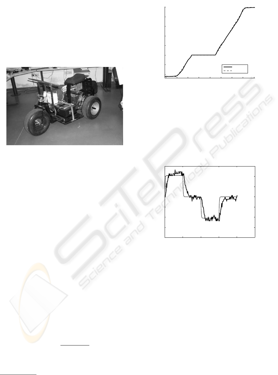
Figure 1: The caddy vehicle.
To realize the caddy control and the setting of the
interface card we will have to figure out an estima-
tion of the behavior of the different components that
compose the vehicle.
The caddy can be split into two independent sub-
systems:
• Driver + traction motor
• Linear actuator driver + steering
Concerning the subsystem driver + traction motor,
the manufacturer endows the caddy with an input-
output characteristic derived in no load condition (i.e.
without a passenger). To verify the coherence with
real data we have designed a program test imple-
mented on the interface card. In this test we have fur-
nished various torque steps as inputs to the driver of
the motor and we have measured the velocity with a
100 Hz sampling frequency. We have distributed in
a quite uniform way the voltage interval 0-5 Volt into
the digital range 0-255, with a little more dense fitting
in proximity of the bends. As a result we have ob-
tained a fairly good approximation of the ideal char-
acteristic (see Figure 2), but this however fails if we
consider, for example, a passenger.
As regards the transfer function, the manufacturer
provides the following first order model:
G(s) =
1
1.8s + 22.7
(1)
By comparing the output of this model with the
real outputs measured in different operating condi-
tions (with or without passenger) with respect to the
3
By courtesy of Tekel Instruments Srl, Torino, Italy
60 80 100 120 140 160 180 200 220
−1
−0.5
0
0.5
1
1.5
2
2.5
division (VOLT)
m/s
Speed vs Voltage
Real case
ldeal casel
Figure 2: Ideal and real input\output characteristic in no
load condition.
same inputs (random sequence of steps), it turns out
from the analysis of data that the description of the
dynamic behavior of the system is not satisfying. The
gap increases in presence of a passenger and in the
case of motion on grass (see Figures 3 and 4).
0 5 10 15 20 25
−0.4
−0.3
−0.2
−0.1
0
0.1
0.2
0.3
time (sec)
speed (m/s)
Model validation
Figure 3: Asphalt test with passenger (thin: first order
model response, thick: real response).
In order to achieve a better description of the dy-
namics of the caddy, an identification procedure is
needed.
3 THE MODULATING
FUNCTIONS IDENTIFICATION
By means of input-output data analysis we are look-
ing for a computation of a linear model for the caddy.
The structure of this model must be as simple as pos-
sible (i.e. with a minimum order).
The measured output signal presents a non negli-
gible noise component and there are also unwelcome
variations due to the unevennesses of the ground. For
ICINCO 2005 - SIGNAL PROCESSING, SYSTEMS MODELING AND CONTROL
212

0 5 10 15 20 25
−0.4
−0.3
−0.2
−0.1
0
0.1
0.2
0.3
time (sec)
speed (m/s)
Model validation
Figure 4: Grass test without passenger (thin: first order
model response, thick: real response)
this reason, an identification procedure capable to ex-
tract reliable models even in these conditions is nec-
essary.
3.1 The modulating functions
Consider continuous n-th order linear processes mod-
eled by the following differential equation:
n
X
i=0
b
i
d
i
y(t)
dt
i
=
m
X
i=0
a
i
d
i
u(t)
dt
i
(2)
where u(t) is the input signal and y(t) the output one.
The coefficients a
i
and b
i
are the unknows of the sys-
tem.
Now define a set of smooth functions Φ(t) having
the following properties:
Φ(t) =
Φ(t) t ∈ [0, T]
0 t 6∈ [0, T ]
(3)
∃
d
i
Φ
dt
i
, ∀i = 1, . . . , p, p ≥ n (4)
Φ
(i)
(0) = Φ
(i)
(T ) = 0, i ≤ n. (5)
The time interval I = [0, T ] is commonly named
integration window. We thus denote modulating func-
tions Φ(t) function along with with its derivatives.
Multiplying both members of (2) by Φ(t) and inte-
grating over I we have:
n
X
i=0
b
i
Z
T
0
Φ(t)y
(i)
(t)dt =
=
m
X
i=0
a
i
Z
T
0
Φ(t)u
(i)
(t)dt (6)
Applying the integration by parts rule and keeping the
property 5 in mind, we get:
n
X
i=0
(−1)
i
b
i
Z
T
0
Φ
(i)
(t)y(t)dt =
=
m
X
i=0
(−1)
i
a
i
Z
T
0
Φ
(i)
(t)u(t)dt (7)
The previous statement is an algebraic equation.
The unknows are the coefficients of (2) and the gen-
eral solution is:
α
i
= (−1)
i
Z
T
0
Φ
(i)
(t)y(t)dt (8)
β
i
= (−1)
i
Z
T
0
Φ
(i)
(t)u(t)dt (9)
Without loss of generality we assume:
b
0
= 1 (10)
Therefore, in order to determine all the unknown pa-
rameters a
i
and b
i
, at least n + m + 1 linearly in-
dependent equations are required. These equations
can be generated discretely by shifting the modulat-
ing function along the measured input-output data. In
this manner we obtain the following linear algebraic
system:
Az = c (11)
where z is the vector of unknown parameters. The
matrix A and the vector c consist of terms depending
on the coefficients α
i
and β
i
:
A =
"
α
0,1
. . . α
m,1
−β
1,1
· · · − β
n,1
. . . . . .
α
0,k
. . . α
m,k
−β
1,k
· · · − β
n,k
#
(12)
c = [β
0,1
. . . β
0,k
]
T
(13)
with k ≥ n + m + 1.
If the equation’s number is greater than the number
of unknown parameters, a pseudoinverse solution can
be determined.
Summarizing, the most important features of this
technique are:
• the identification process occurs directly in the time
domain;
• the knowledge of time derivatives of the input and
the output is not necessary;
• the integral nature of the procedure cuts the high
frequency dynamics: the bandwidth is 1/T .
Due to good filtering characteristics and easiness
of implementation, the most popular class of modular
functions is the class of spline functions introduced
by Maletinsky (see (Maletinsky, 1978), (Maletinsky,
1979)). In Figure 5 we are showing some examples
of spline functions.
IDENTIFICATION OF A CAR-LIKE VEHICLE via MODULATING FUNCTIONS
213
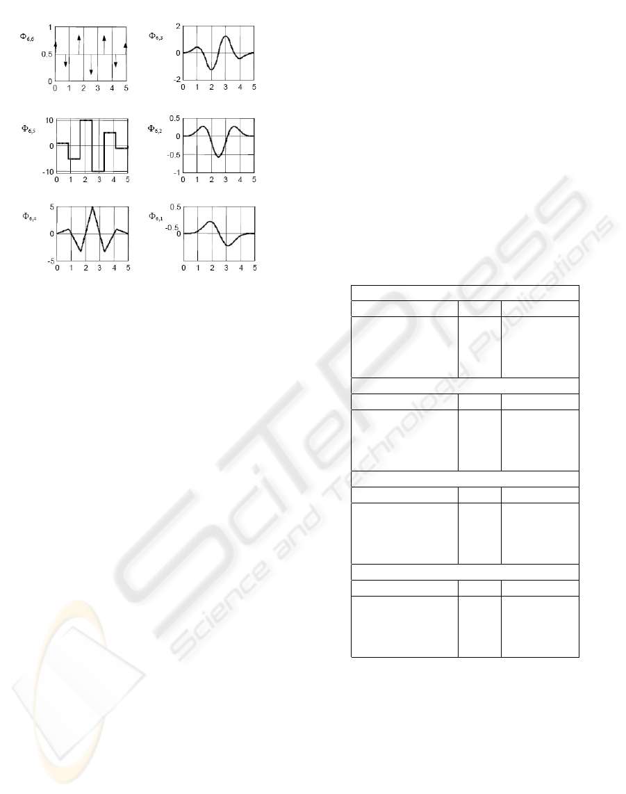
Figure 5: Spline functions of order 6.
Set now as operating point the condition in which
the caddy receives the constant input U = U
0
. At the
output terminal a constant signal Y = Y
0
is measured.
In order to apply the modulating function algorithm
the following steps are required:
1. excitation of the system with the input U = U
0
+u.
The u term represents the variation with respect to
the fixed operating point. The u input must excite
all the dynamics of the system;
2. storage of the corresponding output signal Y =
Y
0
+ y, where y is the variation component;
3. computation of u and y from signals U and Y ;
4. selection of the system structure (number of poles
and zeros) and selection of the integration window;
5. identification procedure applied to u and y.
An appropriate set of data is needed for derive a
number of independent equations sufficient for the pa-
rameter’s calculation.
3.2 The Identification Procedure
The likely operating conditions that we have consid-
ered are are the following:
1. Dry asphalt;
2. Dry asphalt with load (passenger);
3. Grass;
4. Grass with load.
The reference input is U
0
= 170 (digital scale). For
each operative condition several data-sets have been
acquired for different input signals u and a validation
data-set have been selected.
The input signal has been built with rectangular
pulses of variable amplitude. The duration of the
pulses changes along the data sets.
Different models have been obtained for each data
set and have then been compared to the validation
data-set of the corresponding operating condition. For
this purpose the measured output has been compared
to the predicted output of the model and the mean
square error has been computed.
The models have been obtained by different model
structure (number of poles and zeros) and different
amplitude of the integration window. Some examples
are shown in Table 1.
Table 1: Examples of different identifications. Only the best
models with respect to the integrator window T are listed.
Operating condition 1
Model Structure T (s) MSE (m/s)
1 pole 4 0.04
2 poles 2.5 0.02
2 poles, 1 zero 2 0.03
manufacturer - 0.12
Operating condition 2
Model Structure T (s) MSE (m/s)
1 pole 5 0.036
2 poles 3.5 0.024
2 poles, 1 zero 3.5 0.038
manufacturer - 0.122
Operating condition 3
Model Structure T (s) MSE (m/s)
1 pole 4.5 0.054
2 poles 3.5 0.048
2 poles, 1 zero 2.5 0.054
manufacturer - 0.121
Operating condition 4
Model Structure T (s) MSE (m/s)
1 pole 4 0.054
2 poles 4.5 0.049
2 poles, 1 zero 2 0.049
manufacturer - 0.119
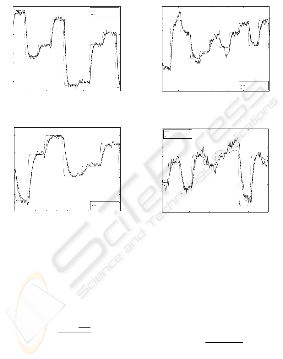
The examples are related to the data sets showing
the features depicted in Table 2. In figures 6-9 it is
shown a comparison with real data.
In terms of mean square error, good results are ob-
tained even with simple models such as second order
transfer function with or without zero. In our case
the presence of the zero does not change significantly
the mean square error; therefore, for the sake of sim-
plicity, we can select the second order model without
zero.
The application of the delay version of modulating
function algorithm (Balestrino et al., 2000) does not
have shown any remarkable delay.
ICINCO 2005 - SIGNAL PROCESSING, SYSTEMS MODELING AND CONTROL
214
10 15 20 25 30 35
−0.4
−0.3
−0.2
−0.1
0
0.1
0.2
0.3
0.4
0.5
Operating condition 1
time (s)
v (m/s)
Real Data
Identified Model
Manufacturer Model
Figure 6: Operating Condition 1.
0 2 4 6 8 10 12 14 16 18 20
−0.5
−0.4
−0.3
−0.2
−0.1
0
0.1
0.2
0.3
0.4
0.5
Operating condition 2
time (s)
v (m/s)
Real Data
Identified Model
Manufacturer Model
Figure 7: Operating Condition 2.
4 BASIS FOR ROBUST CONTROL
Thanks to previous analysis, we currently own a set of
maps describing the behavior of the vehicle in differ-
ent conditions. The basic idea is the construction of a
mean model, that, for our purposes, plays the role of
nominal plant. For this aim a very simple approach is
followed: a mean model is derived for every operating
condition and after the final mean model is computed
as a mean of these results:
z
0
=
N
op
X
j=1
P
N
test
i=1
z
ij
N
test
N
op
(14)
where N
op
is the number of operating conditions (dry
asphalt with or without a person on board, dry grass
with or without a person on board, etc.), N
test
is the
number of models derived in different tests in a given
operating condition.
The term ”uncertainty” refers to the differences or
errors between models and reality. For this reason
5 10 15 20 25 30 35
−0.8
−0.6
−0.4
−0.2
0
0.2
0.4
0.6
Operating condition 3
time (s)
v (m/s)
Real Data
Identified Model
Manufacturer Model
Figure 8: Operating Condition 3.
5 10 15 20 25 30
−0.5
−0.4
−0.3
−0.2
−0.1
0
0.1
0.2
0.3
0.4
Operating condition 4
time (s)
v (m/s)
Real Data
Identified Model
Manufacturer Model
Figure 9: Operating Condition 4.
we are defining uncertainties the deviations with re-
spect to the mean model (14) of all models computed.
The structured representation of uncertainty in the so-
called multiplicative form is (Zhou and Doyle, 1998):
P
∆
= (I + W
m
(s)∆
m
(s))P
0
(s) (15)
where W
m
(s) is a stable transfer matrix describing
the spatial and frequency structure of uncertainty. In
this manner P
∆
is confined in a normalized neighbor-
hood of the nominal plant P
0
(s). For every model
derived in Section 2 the multiplicative uncertainty is
defined as:
∆
im
(s) =
G
i
(s) − G
0
(s)
G
0
(s)
(16)
We then look for a weight transfer function W
m
such
that:
|W
m
(jω)| ≥ |∆
im
(jω)|
In our case the function W
m
(s) is also proper since
G
0
(s) and G
i
(s) have the same relative degrees. Ap-
plying this procedure to the data set, we can find the
IDENTIFICATION OF A CAR-LIKE VEHICLE via MODULATING FUNCTIONS
215
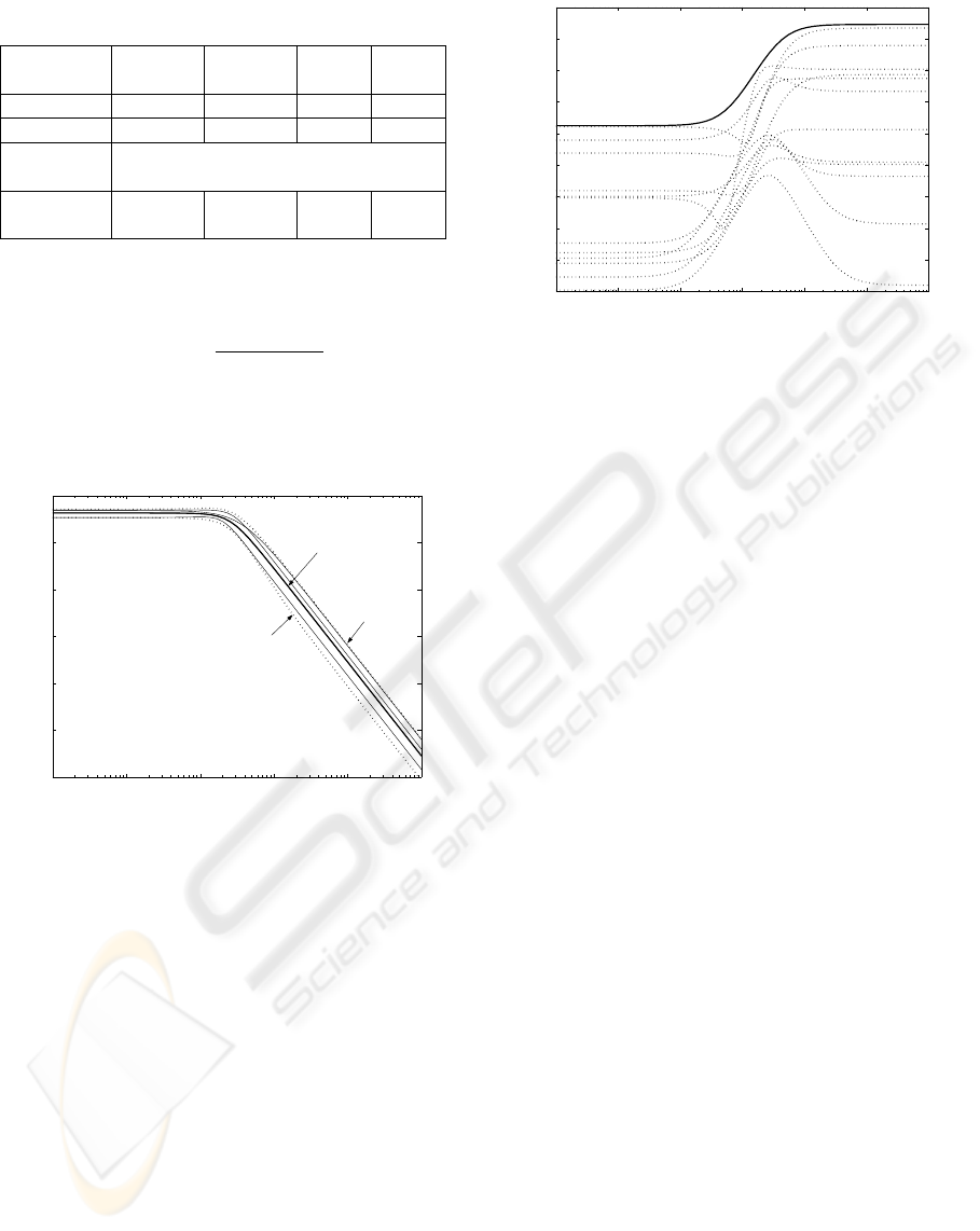
Table 2: Data set features.
Operating
Mode
1 2 3 4
surface Asphalt Asphalt Grass Grass
Passenger No Yes No Yes
Min/Max
step
-10/+10
Step du-
ration (s)
1.5 1.5 2 2
following result:
W
m
(s) =
1.3(s + 0.6)
(s + 3.8)
In Figure 10 the bounded region including all the
models is shown, whereas in Figure 11 the frequency
response of the W
m
(jω) and ∆
im
(jω) is reported.
10
−2
10
−1
10
0
10
1
10
2
10
3
−140
−120
−100
−80
−60
−40
−20
Frequency (rad/sec)
Magnitude (dB)
Nominal Model
Lower Bound
Upper Bound
Figure 10: Bounding region of P
∆
= [1 +
W
m
(s)∆(s)]P
0
(s)
5 ONLINE IDENTIFICATION
The offline version of the modulating function tech-
nique has been used to estimate uncertainties with re-
spect to the chosen nominal model. In order to obtain
a likely uncertain model several tests are necessary.
An online version of this technique can be easily
implemented (Balestrino et al., 2004). In this way an
alternative approach for the control design, based on
adaptive method, seems to be possible. The design of
the controller will require an analysis of the conver-
gence of the method.
To perform the online version of modulating func-
tions algorithm we will have to choose:
• The model structure;
• The number of rows of the A matrix defined in 12;
10
−3
10
−2
10
−1
10
0
10
1
10
2
10
3
−40
−35
−30
−25
−20
−15
−10
−5
0
5
Frequency (rad/sec)
Magnitude (dB)
Figure 11: ∆
im
(dashed lines) and the bound
W
m
(solid line).
• The integration window duration(T);
• An initial estimation of z (given, for example, by a
offline procedure);
Input-output data are stored continuously. Every T
seconds a new equation is generated using (7) and the
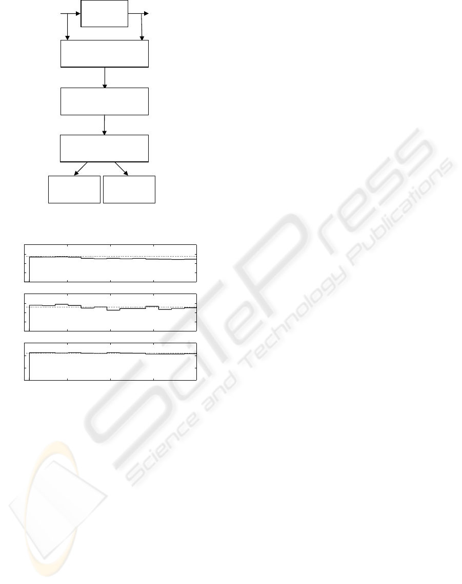
following steps are performed (see Figure 12):
1. Starting from the previous matrix A
k−1
and the
vector c
k−1
, the A
k
matrix and the vector c
k
are
updated with a First In First Out strategy taking in
account the new equation;
2. The following index is calculated:
∆ = kA
k
z
k−1
− c
k
k (17)
were z
k−1
is the previous parameter’s vector;
3. If ∆ > ǫ, where ǫ is a fixed positive threshold,
then the new row brings meaningful new informa-
tion and the algorithm can proceed to the next step.
Otherwise, the A
k−1
and c
k−1
are restored and the
algorithm returns to step 1;
4. computation of the new z
k
. Return to step 1.
It is worth to notice that, in order to increase the
frequency of the parameter’s computation, the inte-
gration windows can overlap. In Figure 13 we are
showing the application of the online algorithm in dry
asphalt operating mode.
6 CONCLUSION
The modulating functions technique guarantees the
identification of a second order linear model, which
thoroughly describes the dynamics of a caddy vehicle.
The offline classic version of the procedure allows to
set the control problem for unmanned guidance from
the point of view of robustness. The online version
of the technique enables an adaptive control strategy.
ICINCO 2005 - SIGNAL PROCESSING, SYSTEMS MODELING AND CONTROL
216
U
Y
Caddy
Modulation
Matrix
Update
Data Check:
useful information ?
Update
Model
Model
hold
Yes
No
Figure 12: Block diagram of online algorithm.
15 20 25 30 35
0
0.2
0.4
0.6
0.8
b
2
15 20 25 30 35
0
0.05
0.1
0.15
0.2
b
1
15 20 25 30 35
0
0.02
0.04
0.06
time (s)
k
Figure 13: Second order model in dry asphalt: Offline pa-
rameters (dashed line), Online parameters (solid line).
Our intent in a near future is the design and the im-
plementation of controllers following the guidelines
showed in this work.
ACKNOWLEDGEMENT
The authors would like to express their sincere appre-
ciations to Roberto Mati, Manuele Cellini and Luca
Greco for their technical support and their gratitude
to Prof. Aldo Balestrino for his advices.
REFERENCES
Balestrino, A., Bolognesi, P., Landi, A., and Sani, L. (2004).
Fault detection of pm synchronous motor via modu-
lating functions. In Symposium on Power Electronics,
Electrical Drives, Automation & Motion, SPEEDAM.
Balestrino, A., Landi, A., and Sani, L. (2000). Para-
meter identification of continuous systems with mul-
tiple input time delays via modulating functions.
IEE Proceedings on Control Theory & Applications,
147(1):19–27.
Balestrino, A., Landi, A., and Sani, L. (2003). Large sig-
nal models of zvs class E
2
resonant converters. In
10th European Conference on Power Electronics and
Applications.
Daniel-Berhet, S. and Unbehauen, H. (1996). Application
of the hartley modulating functions method for the
identification of the bilinear dynamics of a dc motor.
In 35th Conference on Decision and Control.
Daniel-Berhet, S. and Unbehauen, H. (1997). Physical para-
meter estimation of the nonlinear dynamics of a single
link robotic manipulator with flexible joint using the
hmf-method. In Proceedings of the American Control
Conference.
Maletinsky, V. (1978). Identification kontinuierlicher dy-
namischer prozesse. PhD thesis, ETH Zurich.
Maletinsky, V. (1979). Identification of continuous dy-
namical system with spline-type modulating function
method. In IFAC Congr. On Parameter Identification
and Parameter Estimation.
Pearson, A. E. (1992). Explicit parameter identification for
a class of nonlinear input/output differential operator
models. In 31st Conference On Decision And Control.
Shinbrot, M. (1957). On the analysis of linear and non linear
systems. Trans. ASME, 79:547–552.
Zhou, K. and Doyle, J. C. (1998). Essentials of robust con-
trol. Prentice Hall.
IDENTIFICATION OF A CAR-LIKE VEHICLE via MODULATING FUNCTIONS
217
