
REAL-TIME TIME-OPTIMAL CONTROL FOR A NONLINEAR
CONTAINER CRANE USING A NEURAL NETWORK
T.J.J. van den Boom, J.B. Klaassens and R. Meiland
Delft Center for Systems and Control
Mekelweg 2, 2628 CD Delft, The Netherlands
Keywords:
Time-optimal crane control, Nonlinear Model Predictive Control, Optimization, binary search algorithm,
neural networks, Bayesian regularization.
Abstract:
This paper considers time-optimal control for a container crane based on a Model Predictive Control approach.
The model we use is nonlinear and it is planar, i.e. we only consider the swing (not the skew) and we take
constraints on the input signal into consideration. Since the time required for the optimization makes time-
optimal not suitable for fast systems and/or complex systems, such as the crane system we consider, we
propose an off-line computation of the control law by using a neural network. After the neural network has
been trained off-line, it can then be used in an on-line mode as a feedback control strategy.
1 INTRODUCTION
The need for fast transport of containers from quay
to ship and from ship to quay, is growing more and
more. Since ships and their container capacity grow
larger, a more time efficient manner of (un)loading
containers is required. Shipping companies focus on
maximizing the sailing hours and reducing the hours
spent in port. A longer stay in port will eliminate the
profit gained at sea for the large vessels and can hardly
be considered as an option.
Much research has been done on the crane mod-
elling and control (Marttinen et al., 1990),(Fliess
et al., 1991),(H
¨
am
¨
al
¨
ainen et al., 1995), (Bartolini
et al., 2002), (Giua et al., 1999) however most mod-
els are linearized. In this paper we study time-optimal
control for a container crane using a nonlinear model.
The drawback of time-optimal control, in the pres-
ence of constraints, is its demand with respect to
computational complexity. This doesn’t make time-
optimal control suitable for fast systems, such as the
crane system. To overcome this problem a neural
network can be used. It can be trained off-line to
’learn’ the control law obtained by the time-optimal
controller. After the neural network has been trained
off-line, it can then be used in an on-line mode as a
feedback control strategy. In Nonlinear Model Pre-
dictive Control (MPC) an off-line computation of the
control law using a feed-forward neural network was
already proposed by (Parisini and Zoppoli, 1995).
The off-line approach was also followed in (Pottman
and Seborg, 1997), where a radial basis function net-
work was used to ‘memorize’ the control actions. In
this paper we extend these ideas to time-optimal con-
trol.
Section 2 describes the continuous-time model of
the crane and the conversion from the continuous-
time model to a discrete-time model. Section 3 dis-
cusses time-optimal control. Section 4 gives an out-
line of a feedforward network and discuss the best ar-
chitecture of the neural network with respect to the
provided training data. Section 5 gives conclusions
about how well the time-optimal controller performs
in real time.
2 CRANE MODEL
A dynamical crane model is presented in this section.
A schematic picture of the container crane is shown
in figure 1. The container is picked up by a spreader,
which is connected to a trolley by the hoisting cables.
One drive in controlling the motion of the trolley and
another drive is controlling the hoisting mechanism.
The electrical machines produce the force F
T
acting
on the trolley and the hoisting force F
H
and providing
the motion of the load. The dynamics of the electrical
motors is not included in the model. The combina-
39
J. J. van den Boom T., B. Klaassens J. and Meiland R. (2005).
REAL-TIME TIME-OPTIMAL CONTROL FOR A NONLINEAR CONTAINER CRANE USING A NEURAL NETWORK.
In Proceedings of the Second International Conference on Informatics in Control, Automation and Robotics, pages 39-44
DOI: 10.5220/0001179800390044
Copyright
c
SciTePress
tion of the trolley and the container is identified as a
two-sided pendulum. The elastic deformation in the
cables and the crane construction is neglected. The
load (spreader and container) is presented as a mass
m
c
hanging on a massless rope. Friction in the system
is neglected. Only the swing of the container is con-
sidered while other motions like skew are not taken
into account. Further, the sensors are supposed to be
ideal without noise. The influence of wind and sensor
noise can be included in the model as disturbances.
r
r
-
A
A
A
A
A
A
A
A
A
A
A
A
AU
?
-
:
(0, 0)
x
t
Trolley
m
t
θ
F
g
F
T
F
H
ℓ
Container
m
c
Figure 1: Jumbo Container Crane model
The continuous time model is presented by the fol-
lowing equations:
¨x
t
=
m
c
G
h
g sin θ cos θ + m
c
G
h
l
˙
θ
2
sin θ
(m
c
+ G
h
) (m
t
+ G
t
) + G
h
m
c
(1 − cos
2
θ)
+
F
T
(m
c
+ G
h
) − m
c
F
H
sin θ
(m
c
+ G
h
) (m
t
+ G
t
) + G
h
m
c
(1 − cos
2
θ)
(1)
¨
θ =
−¨x
t
cos θ − 2
˙
l
˙
θ − g sin θ
l
(2)
¨
l =
F
H
− m
c
¨x
t
sin θ + m
c
l
˙
θ
2
+ m
c
g cos θ
m
c
+ G
h
(3)
where x
t
is position of the trolley, θ is the swing
angle, l is the length of the cable, m
c
is the container
mass, m
t
is the trolley mass, G
t
is the virtual trolley
motor mass, G
h
is the virtual hoisting motor mass,
F
T
transversal force and F
H
is the hoisting force.
By defining the following state and control signals
z =
x
t
˙x
t
θ
˙
θ
l
˙
l
, u =
F
T
(F
H
− F
H0
)
,
where F
H0
= −m
c
g is used to compensate gravity
of the container, we obtain the continuous dynamic
system in the following form:
˙z(t) = f (z(t), u(t)) (4)
Discrete-time model
Since the controller we will use is discrete, a discrete-
time model is needed. We have chosen Euler’s
method because it is a fast method. The Euler ap-
proximation is given by:
z(k + 1) = z(k ) + T · f (k, z(k), u(k)) (5)
where the integration interval △t is the sampling time
T .
3 TIME-OPTIMAL CONTROL
In this paper we consider time-optimal control for
the crane. Some papers recommend the planning of
a time-optimal trajectory and use this as a reference
path for the container to follow ((Gao and Chen,
1997), (Kiss et al., 2000), (Klaassens et al., 1999)).
We have chosen not to determine a pre-calculated
time-optimal path and subsequently use this as a
reference, in stead we calculate the time-optimal path
using a two step iteration. In a first step we propose a
specific time interval N and evaluate if there is a fea-
sible solution that brings the container to the desired
end-position (x
c,des
, y
c,des
) within the proposed time
interval N . In the second step we enlarge the time
interval if no feasible solution exists, or we shrink
the interval if there is a feasible solution. We iterate
over step 1 and step 2 until we find the smallest time
interval N
opt
for which there exists a feasible solution.
First step:
To decide, within the first step, whether there is a fea-
sible solution for a given time interval N , we min-
imize a Model Predictive Control (MPC) type cost-
criterion J(u, k) with respect to the time interval con-
straint and additional constraint for a smooth opera-
tion of the crane. In MPC we consider the future evo-
lution of the system over a given prediction period
[k + 1, k + N
p
], which is characterized by the predic-
tion horizon N
p
(which is much larger than the pro-
posed time interval), and where k is the current sam-
ple step. For the system (5) we can make an estimate
ICINCO 2005 - INTELLIGENT CONTROL SYSTEMS AND OPTIMIZATION
40

ˆz(k + j) of the output at sample step k + j based on
the state z(k) at step k and the future input sequence
u(k), u(k + 1), . . . , u(k + j − 1). Using successive
substitution, we obtain an expression of the form
ˆz(k+j) = F
j
(z(k), u(k), u(k+1), . . . , u(k+j−1))
for j = 1, . . . , N
p
. If we define the vectors
˜u(k) =
u
T
(k) . . . u
T
(k + N
p
− 1)
T
(6)
˜z(k) =
ˆz(k + 1) . . . ˆz(k + N
p
)
T
, (7)
we obtain the following prediction equation:
˜z(k) =
˜
F (z(k), ˜u(k)) . (8)
The cost criterion J(u, k) used in MPC reflects the
reference tracking error (J
out
(˜u, k)) and the control
effort (J
in
(˜u, k)):
J(˜u, k) = J
out
(˜u, k) (k) + λJ
in
(˜u, k) (k)
=
N
p
X
j=1
|ˆx
c
(k+j) − x
c,des
|
2
+ |ˆy
c
(k+j) − y
c,des
|
2
+ λ|u(k + j − 1)|
2
(9)
where x
c
= ˆz
1
+ ˆz
5
sin ˆz
3
is the x-position of the
container, y
c
= ˆz
5
cos ˆz
3
is the y-position of the
container, and λ is a nonnegative integer. From the
above it is clear that J(k ) is a function of ˜z(k ) and
˜u(k), and so is a function of z(k) and ˜u(k).
In practical situations, there will be constraints on
the input forces applied to the crane:
−F
T max
≤ u
1
≤ F
T max
,
F
H max
− F
H0
≤ u
2
≤ −F
H0
.
(10)
where, because of the sign of F
H
, we have F
H max
<
0 and F
H0
= −m
c
g < 0. Further we have the time
interval constraints that
|ˆx
c
(N + i) − x
c,des
| ≤ ǫ
x
, i ≥ 0
|ˆy
c
(N + i) − y
c,des
| ≤ ǫ
y
, i ≥ 0
(11)
which means that at the end of the time interval N
the container must be at its destination with a desired
precision ǫ
x
and ǫ
y
, respectively.
Consider the constrained optimization problem to
find at time step k a ˜u(k) where:
˜u
∗
(k) = arg min
˜u
J (˜u, k)
subject to (10) and (11). Note that the above opti-
mization is a nonlinear optimization with constraints.
To reduce calculation time for the optimization we
can rewrite the constrained optimization problem into
an unconstrained optimization problem by introduc-
ing auxiliary input variables for the force constraints
and penalty functions to account for the time interval
constraint. For the force constraints we consider the
auxiliary inputs v
1
and v
2
:
u
1
= α arctan
v
1
α
u
2
=
β arctan
v
2
β
, v
2
< 0
v
2
, 0 < v
2
< (βπ/2)
γ + β arctan
v
2
−γ
β
, v
2
> (βπ/2)
where α = 2F
T max
/π, β = 2(F
H max
− F
H0
)/π and
γ = F
H max
− 2F
H0
. Note that for all v
1
, v
2
∈ R
input force constraints (10) will be satisfied.
For the time interval constraints we define the
penalty function:
J
pen
(˜u, k) =
N
p
X
j=N −k
µ|ˆx
c
(k+j) − x
c,des
|
2
+µ|ˆy
c
(k+j) − y
c,des
|
2
(12)
where µ ≫ 1. Beyond the time interval (so for k+j ≥
N) the influence of any deviation from the desired
end point is large and the container position and speed
must then be very accurate.
Instead of the constrained optimization problem we
have now recast the problem as an unconstrained op-
timization problem at time step k:
˜v
∗
(k) = arg min
˜v
J (˜u(˜v), k) + J
pen
(˜u(˜v), k)
where
˜v(k) =
v
T
(k) . . . v
T
(k + N
p
− 1)
T
For the optimization we use an iterative optimization
algorithm where in each iteration step we first select
a search direction and then we perform a line search,
i.e., an optimization along the search direction. The
search direction is according the Broyden-Fletcher-
Goldfarb-Shanno method and for the line search we
have chosen a mixed quadratic and cubic polynomial
method.
Second step:
In the first step we have a constant penalty function
shifting point N, which has to be chosen differently
for every different initial state and steady state. When
we have chosen a value for N for a certain initial state
and steady state such that the states converge, we can
lower the value of N. On the other hand, when we
have chosen a value for N for a certain initial state
and steady state such that the states do not converge
within the allowed region, we have to increase the
value of N. When we have found the optimal value
N = N
opt
if for N there exists a feasible solution,
and reduction of N will lead to an infeasible prob-
lem. In other words, The determination of N
opt
has
REAL-TIME TIME-OPTIMAL CONTROL FOR A NONLINEAR CONTAINER CRANE USING A NEURAL
NETWORK
41

become a feasibility study. To determine the optimal
value N
opt
for each different initial state z
0
and steady
state (x
c,des
, y
c,des
) in an efficient way, we have im-
plemented a simple binary search algorithm.
4 NEURAL NETWORK
Since the time required for the optimization makes
time-optimal control not suitable for fast systems, we
propose an off-line computation of the control law us-
ing a neural network. We assume the existence of
a function that maps the state to the optimal control
action, and this function is continuous. Continuous
functions can be approximated to any degree of ac-
curacy on a given compact set by feedforward neural
networks based on sigmoidal functions, provided that
the number of neural units is sufficiently large. How-
ever, this assumption is only valid if the solution to the
optimization problem is unique. After the neural net-
work controller has been constructed off-line, it can
then be used in an on-line mode as a feedback control
strategy. Because the network will always be an ap-
proximation, it cannot be guaranteed that constraints
are not violated. However, input constraints, which
are the only constraints we consider, can always be
satisfied by limiting the output of the network.
Training of the neural network
We have covered the workspace of the crane as can
be seen in Table 1. We have considered all initial
Table 1: Values of x
0
and x
des
x
t
0
= 0 [m]
x
t,des
= {0, 5, 10, . . . , 60} [m]
l
0
= {5, 10, 15, . . . , 50} [m]
l
des
= {5, 10, 15, . . . , 50} [m]
speeds zero, i.e. ˙x
t
0
,
˙
θ
0
,
˙
l
0
as well as the swing an-
gle θ
0
are zero. The initial state for the trolley, x
t
0
, is
always zero, and the steady state is within the range
0 ≤ x
t,des
≤ 60 m , with steps of 5 m. The dynamical
behavior of the crane depends on the distance of the
trolley travelling x
t
− x
t,des
and not on its position.
This explains why we only consider x
t
0
= 0 m.
We don’t consider simulations where we start and
end in the same states, or in other words, where we
stay in equilibrium. Thus the total amount of different
combinations of initial states x
0
and steady states x
des
is 13 × 10 × 10 − 10 = 1290.
It is of utmost importance to keep the number of
inputs and outputs of the neural network as low as
possible. This to avoid unnecessary complexity with
respect to the architecture of the neural network. No-
tice that most of the steady states we use for the con-
trol problem, are always zero and can be disregarded
for the input signal of the neural network. The only
exceptions are x
t,des
and l
des
. Furthermore, we can
reduce the number of inputs by taking the distance of
the trolley travelling x
t
− x
t,des
, while still providing
the same dynamic behavior. We cannot reduce the
number of the outputs, hence for the minimum num-
ber of inputs (z) and outputs (y) we have:
z =
x
t
− x
t,des
˙x
t
θ
˙
θ
l
˙
l
l
des
, u =
u
1
u
2
We can reduce the dimension of the input vector
even more by using principal component analysis as a
preprocessing strategy. We eliminate those principal
components which contribute less than 2 percent. The
result is that the total number of inputs now is 6 in
stead of 7.
We have trained the neural network off-line with
the Levenberg-Marquardt algorithm. We have used
one hidden layer and we have used Bayesian regu-
larization to determine the optimal setting of hidden
neurons. For more detail about Bayesian regulariza-
tion we refer to (Mackay, 1992) and (Foresee and Ha-
gan, 1997).
Table 2: Bayesian regularization results for a 6-m
1
-2 feed-
forward network
m
1
E
T r
E
T st
E
V al
E
w
W
eff
5 42318 26759 14182 176 46.9
10 34463 29379 11568 226 90.6
20 24796 32502 8425 2164 180
30 24318 32819 8270 1219 268
40 21636 33573 7411 1099 357
50 18726 34617 6420 2270 445
60 19830 34152 6831 813 535
70 3462 7315 1424 1453 618
80 3599 7350 1473 828 704
90 3337 7459 1409 1232 793
100 3404 7473 1459 923 875
110 3225 7371 1401 1100 964
120 3237 7401 1437 1005 1046
130 3512 7281 1415 982 977
For the results we refer to Table 2 where m
1
de-
notes the number of neurons of the first (and only)
hidden layer, E
T r
, E
T st
and E
V al
denote the sum of
squared errors on the training subset, test subset and
on the validation subset respectively. The sum of
ICINCO 2005 - INTELLIGENT CONTROL SYSTEMS AND OPTIMIZATION
42
0 5 10 15 20
0
20
40
0 5 10 15 20
−5
0
5
0 5 10 15 20
−0.2
0
0.2
0 5 10 15 20
−0.2
0
0.2
0 5 10 15 20
0
20
40
0 5 10 15 20
−5
0
5
0 5 10 15 20
0
20
40
0 5 10 15 20
−5
0
5
0 5 10 15 20
0
20
40
0 5 10 15 20
−5
0
5
0 5 10 15 20
−1
0
1
0 5 10 15 20
0
2
4
x
t
(m)
˙x
t
(m/s)
θ (rad)
˙
θ (rad/s)
l (m)
˙
l (m/s)
x
c
(m)
˙x
c
(m/s)
y
c
(m)
˙y
c
(m/s)
T
t
(10
6
Nm)
T
h
(10
6
Nm)
t (s)t (s)
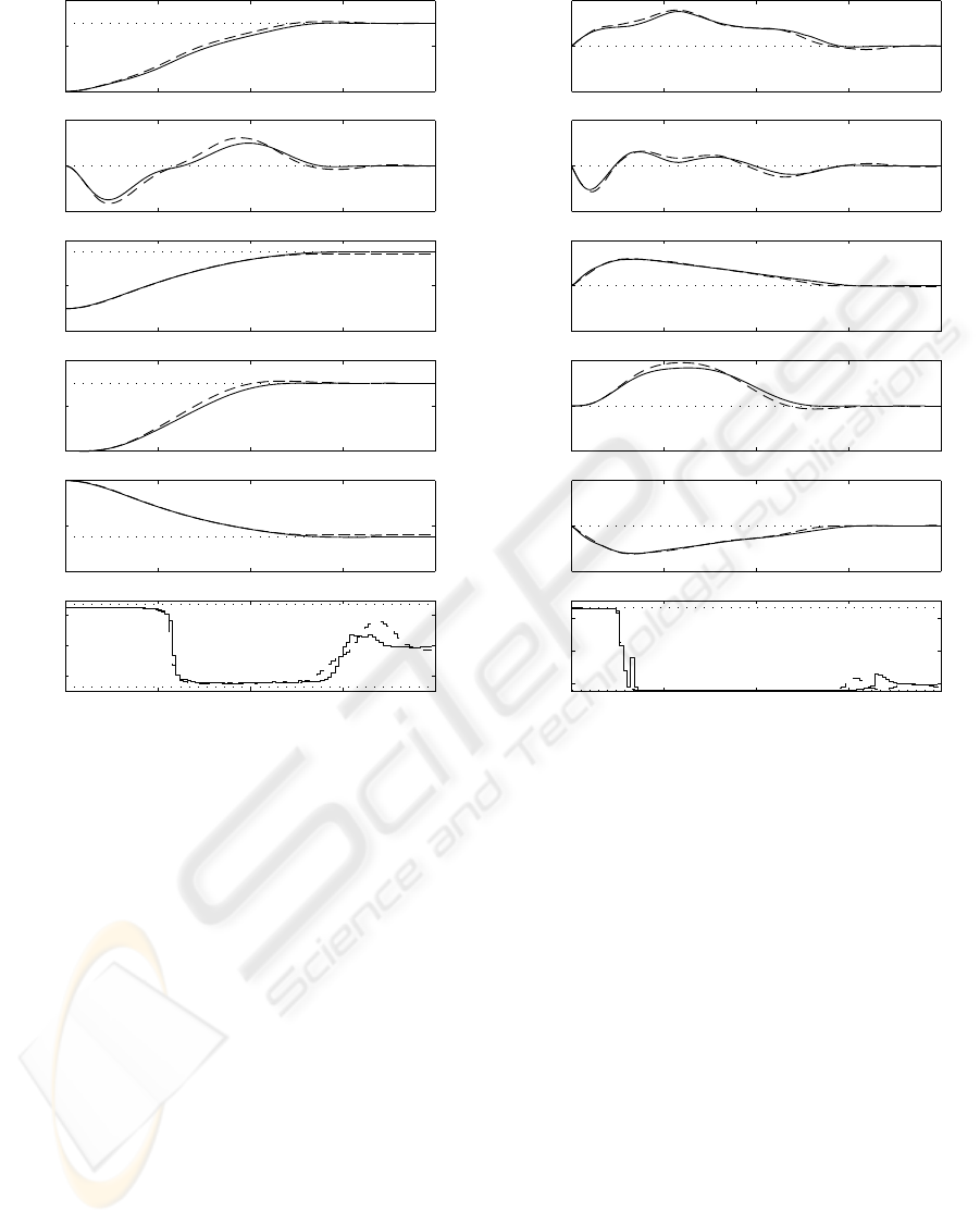
Figure 2: Comparison of simulation results between the time-optimal controller (solid line) and the neural network approxi-
mation (dashed line)
squares on the error weights is denotes by E
w
and
W
eff
is the effective number of parameters.
We have tested the neural network controller as a
feedback control strategy in an online mode. Fig-
ure 2 shows a comparison between the neural net-
work controller and the time-optimal controller where
the dashed line denotes the simulation for the time-
optimal controller and the solid line denotes the
neural network simulation. The result seems satisfac-
tory. The total cpu time of the neural network was
2.5 s and the total cpu time of the time-optimal con-
troller was 17 minutes and 58 seconds. The neural
network controller can easily be implemented in an
online mode as a feedback control strategy.
5 DISCUSSION
In this paper an implementation of a time-optimal
controller for a planar crane system is presented,
based on an MPC approach. A nonlinear state space
system was used for a model and we have imple-
mented on the inputs. We have trained a neural net-
work off-line with the training data obtained from the
time-optimal controller. We have used Bayesian regu-
larization to determine the optimal settings of the total
number of hidden neurons. The trained neural net-
work can be used in an online feedback control strat-
egy.
In future research we will search methods to obtain
the data, necessary for training the neural networks,
in an efficient way, and to avoid redundancy. Further
we will include the skew motion of the container, and
introduce trajectory constraints to prevent collision of
the container with other objects.
REAL-TIME TIME-OPTIMAL CONTROL FOR A NONLINEAR CONTAINER CRANE USING A NEURAL
NETWORK
43

REFERENCES
Bartolini, G., Pisano, A., and Usai, E. (2002). Second-order
sliding-mode control of container cranes. Automatica,
38:1783–1790.
Fliess, M., L
´
evine, J., and Rouchon, P. (1991). A simpli-
fied approach of crane control via a generalized state-
space model. Proceedings of the 30th Conference on
Decision and Control, Brighton, England.
Foresee, F. and Hagan, M. (1997). Gauss-newton approxi-
mation to bayesian learning. Proceedings of the 1997
International Joint Conference on Neural Networks,
pages 1930–1935.
Gao, J. and Chen, D. (1997). Learning control of an over-
head crane for obstacle avoidance. Proceedings of
the American Control Conference, Albuquerque, New
Mexico.
Giua, A., Seatzu, C., and Usai, G. (1999). Oberserver-
controller design for cranes via lyapunov equivalence.
Automatica, 35:669–678.
H
¨
am
¨
al
¨
ainen, J., Marttinen, A., Baharova, L., and
Virkkunen, J. (1995). Optimal path planning for a
trolley crane: fast and smooth transfer of load. IEEE
Proc.-Control Theory Appl., 142(1):51–57.
Kiss, B., L
´
evine, J., and Mullhaupt, P. (2000). Control of a
reduced size model of us navy crane using only motor
position sensors. In: Nonlinear Control in the Year
2000, Editor: Isidori, A., F. Lamnabhi-Lagarrigue and
W. Respondek. Springer, New York, 2000, Vol.2. pp.
1-12.
Klaassens, J., Honderd, G., Azzouzi, A. E., Cheok, K. C.,
and Smid, G. (1999). 3d modeling visualization for
studying control of the jumbo container crane. Pro-
ceedings of the American Control Conference, San
Diego, California, pages 1754–1758.
Mackay, D. (1992). Bayesian interpolation. Neural Com-
putation, 4(3):415–447.
Marttinen, A., Virkkunen, J., and Salminen, R. (1990). Con-
trol study with a pilot crane. IEEE Transactions on
education, 33(3):298–305.
Parisini, T. and Zoppoli, R. (1995). A receding-horizon reg-
ulator for nonlinear systems and a neural approxima-
tion. Automatica, 31(10):1443–1451.
Pottman, M. and Seborg, D. (1997). A nonlinear predictive
control strategy based on radial basis function models.
Comp. Chem. Eng., 21(9):965–980.
ICINCO 2005 - INTELLIGENT CONTROL SYSTEMS AND OPTIMIZATION
44
