
WIND TURBINE ROTOR ACCELERATION: IDENTIFICATION
USING GAUSSIAN REGRESSION
W. E. Leithead
Dept of Electronic and Electrical Engineering, University of Strathclyde, Glasgow, U.K.
and
Hamilton Institute, National University of Ireland, Maynooth, Co. Kildare, Ireland
Yunong Zhang, Kian Seng Neo
Hamilton Institute, National University of Ireland, Maynooth, Co. Kildare, Ireland
Keywords: Data analysis, Gaussian regression, inde
pendent processes, fast algorithms.
Abstract: Gaussian processes prior model methods for data analysis are applied to wind turbine time series data to
identify both rotor speed and rotor acceleration from a poor measurement of rotor speed. In so doing, two
issues are addressed. Firstly, the rotor speed is extracted from a combined rotor speed and generator speed
measurement. A novel adaptation of Gaussian process regression based on two independent processes rather
than a single process is presented. Secondly, efficient algorithms for the manipulation of large matrices are
required. The Toeplitz nature of the matrices is exploited to derive novel fast algorithms for the Gaussian
process methodology that are memory efficient.
1 INTRODUCTION
Following some initial publications in the late 1990s
(e.g., Rasmussen (1996), Gibbs (1997), Mackay
(1998), Williams and Barber (1998)), interest has
grown quickly into the application of Gaussian
process prior models to data analysis; e.g. Williams
(1999), Gibbs and Mackay (2000), Sambu et al
(2000), Toshioka and Ishii (2001), Leith et al
(2002), Shi et al (2003), Solak et al (2003), Leithead
et al (2003a), Leithead et al (2003b). In this paper,
these methods are applied to wind turbine time
series data, specifically, site measurements of the
rotor speed for a commercial 1MW machine.
However, the measurement is some unknown
combination of the rotor speed and the generator
speed (scaled by the gearbox ratio) (Leithead et al,
2003b). Furthermore, the data is corrupted by
significant measurement noise. The objective of the
data analysis is to extract from the data both the
rotor speed and the rotor acceleration, an initial yet
important part of identifying the aerodynamics and
drive-train dynamics of variable speed wind turbines
(Leithead et al, 2003b). Previously, only traditional
filtering methods have been employed (Leithead et
al, 2003b).
To successfully identify the wind turbine rotor
spee
d
and acceleration using Gaussian process prior
models, two particular issues must be addressed.
Firstly, since the measurement is a combination of
rotor speed and generator speed, only that
contribution to the measurement due to the rotor
speed must be extracted. Secondly, since analysis
using Gaussian process prior models involves the
inversion and multiplication of N-dimensional
square matrices where N is the number of data
measurements (24,000 in this case), the matrix
manipulations must be efficient. In this paper, novel
adaptations of the Gaussian process data analysis
methodology to meet these two issues are presented
(the first in section 3 and the second in section 4)
and successfully applied to the wind turbine data (in
section 5).
84
E. Leithead W., Zhang Y. and Seng Neo K. (2005).
WIND TURBINE ROTOR ACCELERATION: IDENTIFICATION USING GAUSSIAN REGRESSION.
In Proceedings of the Second International Conference on Informatics in Control, Automation and Robotics - Signal Processing, Systems Modeling and
Control, pages 84-91
DOI: 10.5220/0001179300840091
Copyright
c
SciTePress

2 GAUSSIAN PROCESS PRIOR
MODELS
Gaussian process prior models and their application
to data analysis is reviewed in theis section.
Consider a smooth scalar function f(.) dependent
on the explanatory variable,
. Suppose
N measurements,
{
, of the value of the
function with additive Gaussian white measurement
noise, i.e. y
p
D ℜ⊆∈z
}
N
1i
ii
)y,(
=
z
i
=f(z
i
)+n
i
,
are available and denote them
by M. It is of interest here to use this data to learn
the mapping f(z) or, more precisely, to determine a
probabilistic description of f(z) on the domain, D,
containing the data. Note that this is a regression
formulation and it is assumed the explanatory
variable, z, is noise free. The probabilistic
description of the function, f(z), adopted is the
stochastic process, f
z
, with the E[f
z
], as z varies,
interpreted to be a fit to f(z). By necessity, to define
the stochastic process, f
z
, the probability
distributions of f
z
for every choice of value of
D
∈
z
are required together with the joint probability
distributions of
for every choice of finite
sample, {z
i
f
z
1
,…,z
k
}, from D, for all k>1. Given the
joint probability distribution for
i
, i=1..N, and the
joint probability distribution for n
f
z
i
, i=1..N, the joint
probability distribution for y
i
, i=1..N, is readily
obtained since the measurement noise, n
i
, and the
f(z
i
) (and so the
i
) are statistically independent. M
is a single event belonging to the joint probability
distribution for y
f
z
i
, i=1..N.
In the Bayesian probability context, the prior
belief is placed directly on the probability
distributions describing f
z
which are then
conditioned on the information, M, to determine the
posterior probability distributions. In particular, in
the Gaussian process prior model, it is assumed that
the prior probability distributions for the f
z
are all
Gaussian with zero mean (in the absence of any
evidence the value of f(z) is as likely to be positive
as negative). To complete the statistical description,
requires only a definition of the covariance function
=E[ , ], for all z
),(C
jif
zz
i
f
z
j
f
z
i
and z
j
. The
resulting posterior probability distributions are also
Gaussian. This model is used to carry out inference
as follows.
Clearly where p(M)
acts as a normalising constant. Hence, with the
Gaussian prior assumption,
M)/p(M),f(p)M|f(p
zz
=
[]
⎥
⎥
⎦
⎤
⎢
⎢
⎣
⎡
⎥
⎦
⎤
⎢
⎣
⎡
⎥
⎥
⎦
⎤
⎢
⎢
⎣
⎡
Λ
−∝
−
Y
Y
z
zz
f
fMfp
1
2221
T
`2111
T
2
1
exp)|(
ΛΛ
Λ
(1)
where
, Λ
T
N
yy ],[
1
"=Y
11
is E[f
z
, f
z
], the ij
th
element of the covariance matrix Λ
22
is E[y
i
, y
j
] and
the i
th
element of vector Λ
21
is E[y
i
, f
z
]. Both Λ
11
and
Λ
21
depend on z. Applying the partitioned matrix
inversion lemma, it follows that
(
)
][ )
ˆ
()
ˆ
(exp|
1
2
1
zzzzzz
ffffMfp −Λ−−∝
−
(2)
with
, .
Therefore, the prediction from this model is that the
most likely value of f(z) is the mean,
, with
variance Λ
Y
z
-1
22
T
21
f
ˆ
ΛΛ=
21
-1
22
T
2111
ΛΛΛ−Λ=Λ
z
z
f
ˆ
z
. Note that is simply a z-dependent
weighted linear combination of the measured data
points, Y, using weights
. The measurement
noise, n
z
f
ˆ
-1
22
T
21
ΛΛ
i
, i=1,..N, is statistically independent of f(z
i
),
i=1,..N, and has covariance matrix B. Hence, the
covariances for the measurements, y
i
, are simply
E[y
i
,y
j
] = E[ , ]+ B
i
f
z
j
f
z
ij
; E[y
i
, f
z
] = E[ , f
i
f
z
z
] (3)
In addition, assume that the related stochastic
process,
, where and e
i
f
e
z
δ
δ−=
δ+
/)f(ff
)(
δ
i
i
zez
e
z
i
is
a unit basis vector, is well-defined in the limit as
0→
δ
, i.e. all the necessary probability
distributions for a complete description exist. Denote
the derivative stochastic process, i.e. the limiting
random process, by
. When the partial derivative
of f(z) in the direction e
i
f
e
z
i
exists, E[ ] as z varies is
interpreted as a fit to
i
f
e
z
δ
)(
z
f
i
z
∂
∂
. Provided the
covariance E[
, ] is sufficiently differentiable,
it is well known (O’Hagan, 1978) that
is itself
Gaussian and that
i
f
z
j
f
z
i
f
e
z
]f[E
z
]f[E
i
i
z
e
z
∂
∂
=
(4)
where z
i
denotes the i
th
element of z; that is, the
expected value of the derivative stochastic process is
just the derivative of the expected value of the
stochastic process. Furthermore,
]f,f[E]f,f[E
]f,f[E]f,f[E
101
i
0
10
j
1
i
0
1
i
2
j
1
i
zzz
e
z
zz
e
z
e
z
∇=
∇∇=
(5)
where
Q(z
1
i
∇
o
,z
1
) denotes the partial derivative of
Q(z
o
,z
1
) with respect to the i
th
element of its first
argument, etc.
WIND TURBINE ROTOR ACCELERATION: IDENTIFICATION USING GAUSSIAN REGRESSION
85
The prior covariance function is generally
dependent on a few hyperparameters,
θ
. To obtain a
model given the data, M, the hyperparameters are
adapted to maximise the likelihood, p(M|
θ
), or
equivalently to minimize the negative log likelihood,
L(
θ
), where
YY
1
)(
2
1
)(detlog
2
1
)(
−
+=
θθθ
CCL
T
(6)
with
22
)( Λ=
θ
C , the covariance matrix of the
measurements.
3 MODELS WITH TWO
GAUSSIAN PROCESSES
Suppose that the measurements are not of a single
function but of the sum of two functions with
different characteristics; that is, the measured values
are y
i
=f(z
i
)+g(z
i
)+n
i
. Now, it is of interest to use the
data to learn the mappings, f(z) and g(z), or, more
precisely, to determine a probabilistic description for
them. The probabilistic description by means of a
single stochastic process, discussed in the previous
section, is no longer adequate. Instead, a novel
probabilistic description in terms of the sum of two
independent stochastic processes, f
z
and g
z
, is
proposed below.
Since f
z
and g
z
are independent, E[FG
T
]=0 where
and . Let the
covariance functions for f
T
]f,f[
N1
zz
F "=
T
]g,g[
N1
zz
G "=
z
and g
z
be and
, respectively. Note that this is a different
model from one using a single stochastic process
with covariance function, (C
),(C
jif
zz
),(C
jig
zz
f
+ C
g
). It follows that
[]
⎥
⎥
⎥
⎦
⎤
⎢
⎢
⎢
⎣
⎡
=
⎥
⎥
⎥
⎦
⎤
⎢
⎢
⎢
⎣
⎡
⎥
⎥
⎥
⎦
⎤
⎢
⎢
⎢
⎣
⎡
=
Q
YGF
Y
G
F
GGFF
GGGG
FFFF
ΛΛ
ΛΛ
ΛΛ
Λ 0
0
E
TTT
(7)
with
, and
.
]E[
T
FF
FF
=Λ ]E[
T
GG
GG
=Λ
GGFF
BQ ΛΛ ++=
The prior joint probability distribution for F, G
and Y is Gaussian with mean zero and covariance
matrix Λ. The requirement is to obtain the posterior
probability distribution for F and G conditioned on
the data set, M, subject to the condition that they
remain independent. Of course, the posterior
probability distribution remains Gaussian. The mean
and covariance matrix for the posterior is provided
by the following theorem (Leithead et al, 2005).
Theorem 1: Given that the prior joint probability
distribution for F, G and Y is Gaussian with mean
zero and covariance matrix Λ, the posterior joint
probability distribution for [F
T
, G
T
]
T
conditioned on
the M, subject to the condition that they remain
independent, is Gaussian with
⎥
⎦
⎤
⎢
⎣
⎡
=
⎥
⎦
⎤
⎢
⎣
⎡
=
−−
−
−−
−
BQBQ
BQ
YQBQ
YQ
GGF
FFF
GGF
FFF
11
1
11
1
0
0
cov
mean
Λ
Λ
Λ
Λ
(8)
where
FFF
BQ
Λ
+
=
.
Proof. Omitted due to space limitations.
Note, since f
z
and g
z
remain independent when
conditioned on M, the prediction and covariance for
(f
z
+g
z
) are simply the sum of the individual
predictions and covariance values.
0 1 2 3 4 5 6 7 8
-4
-3
-2
-1
0
1
2
3
Data, long length-scale prediction and total error
Seconds
Figure 1: Data values (***), long length-scale component
with confidence intervals (––) and total error and
confidence interval (==)
Example: A commonly used prior covariance
function for a Gaussian process with scalar
explanatory variable is
][
2
2
1
)zz(exp
ji
da −−
(9)
It ensures that measurements associated with nearby
values of the explanatory variable should have
higher correlation than more widely separated values
of the explanatory variable;
is related to the
overall mean amplitude and d inversely related to
the length-scale of the Gaussian process.
a
Let the covariance function for f
z
be (9) with
a=1.8 and d=2.5, and the covariance function for g
z
be (9) with a=0.95 and d=120; that is, f
z
has a long
ICINCO 2005 - SIGNAL PROCESSING, SYSTEMS MODELING AND CONTROL
86

length-scale and g
z
a short length-scale. In addition,
let the measurement noise be Gaussian white noise
with variance b=0.04, i.e. B
ij
=b
δ
ij
., where
δ
ij
is the
Kronecker delta. A set of 800 measurements at
constant interval, 0.01, for y
i
=f(z
i
)+g(z
i
)+n
i
, with the
f(z
i
) and g(z
i
) the sample values for the stochastic
processes f
z
and g
z
, respectively, is shown in figure
1.
A prediction for the long and short length-scale
components is obtained using (8); that is, the
conditioning on the data is chosen such that as much
of the data as possible is explained by the long
length-scale component. The long length-scale
component with its confidence interval (
standard
deviations) is shown in Figure 1 and the short
length-scale component with its confidence interval
is shown in Figure 2. The prediction error for (f
2±
z
+g
z
)
with its confidence interval is also depicted in Figure
2.
0 1 2 3 4 5 6 7 8
-2
-1.5
-1
-0.5
0
0.5
1
1.5
2
Short length-scale prediction and confidence intervals
Seconds
Figure 2: Short length-scale component with confidence
intervals
In Section 5, Theorem 1 is applied to the wind
turbine measurement data to extract the contribution
due to the rotor speed and, together with (4) and (5),
to identify the rotor acceleration.
4 TOEPLITZ-BASED
EFFICIENCY IMPROVEMENT
In section 3, a novel adaptation of the Gaussian
regression methodology to support the extraction of
separate components from data is presented.
However, before that procedure can be applied to
large data sets, fast and memory efficient algorithms
are required. That requirement is addressed in this
section.
As the log likelihood, (6), is in general nonlinear
and multimodal, efficient optimisation routines
usually need gradient information,
YY
111
2
1
2
1
−−−
∂
∂
−
⎟
⎟
⎠
⎞
⎜
⎜
⎝
⎛
∂
∂
=
∂
∂
C
C
C
C
Ctr
L
i
T
ii
θθθ
(10)
where
i
θ
denotes the i-th hyperparameter and )(
⋅
tr
the trace operation of a matrix. Let us denote
i
C
θ
∂
∂
/ hereafter by
P
for notational convenience.
Clearly, in general, the number of operations in
solving for
and is of , whilst
the memory space to store
C , and
Cdetlog
1−
C
)(
3
NO
1−
C
P
is
(see Table 1 for specific values). For large
data sets, fast algorithms, that require less memory
allocation, are required for the basic matrix
manipulations,
, and ,
when tuning the Gaussian process prior model
hyperparameters.
)(
2
NO
Cdetlog
yC
1−
)(
1
PCtr
−
Now consider a time series with fixed interval
between the measurements. The explanatory
variable, z, in the Gaussian process prior model is a
scalar, the time t. When the covariance function
depends on the difference in the explanatory
variable, as is almost always the case, the covariance
matrix
)(
θ
C and its derivative matrices
P
are
Toeplitz; that is,
[]
110
021
201
110
)(
−
−−
−
−
=
=
⎥
⎥
⎥
⎥
⎦
⎤
⎢
⎢
⎢
⎢
⎣
⎡
=
N
NN
N
N
cccc
cToeplitz
ccc
ccc
ccc
C
"
"
#%##
"
"
Furthermore,
)(
θ
C is symmetric and positive
definite.
Here, the Toeplitz nature of
)(
θ
C is exploited to
derive novel fast algorithms for the Gaussian process
methodology that require less memory allocation. It
is well-known that positive-definite Toeplitz
matrices can be elegantly manipulated in
operations. For example, Trench's algorithm
inverts
with operations, and Levinson's
algorithm solves for
with operations
(Golub & Van Loan, 1996). However, direct
application of these algorithms to Gaussian process
regression may fail even with medium-scale datasets
due to lack of memory space, see Table 1. For
example, on a Pentium-IV 3GHz 512MB-RAM PC,
)(
2
NO
C 4/13
2
N
yC
1−
2
4N
WIND TURBINE ROTOR ACCELERATION: IDENTIFICATION USING GAUSSIAN REGRESSION
87

a MATLAB-JAVA algorithm usually fails around
because storing almost uses up the
available system memory. The solution is to adapt
the fast algorithms to use only vector-level storage.
From Table 1 that approach is theoretically able to
handle very large datasets, such as 1-million data
points, in terms of memory requirements.
7000=N
1−
C
Table 1: Memory/storage requirement in double precision
N Matrix Vector
1000 7.7 MB 7.6 KB
7000 373.9 MB 53.4 KB
15000 1716.6 MB 114.4 KB
20000 152.6 KB
30000 228.9 KB
50000 381.5 KB
100000 762.9 KB
1000000 7.629 MB
Two versions of fast Toeplitz-computation
algorithms are discussed and compared below;
namely, a full-matrix version and a vector-storage
version.
4.1 Full-Matrix Toeplitz
Computation
The simplest way of applying Toeplitz computation
to Gaussian process regression is to compute
directly as the basis for the other matrix
manipulations. Specifically, Trench's algorithm of
operations can be readily modified to obtain
whilst simultaneously determining as
the logarithm sum of the reflection coefficients.
Then, given
, the computation
1−
C
)(
2
NO
1−
C Cdetlog
1−
C
∑∑
=
−
ij
ijij
pcPCtr )(
1
is easily performed in
operations, where
)(
2
NO
ij
c
and p
ij
are the ij-th
elements of
and P, respectively.
1−
C
Table 2: Accuracy and speedup of Toeplitz computation
N=1000 N=2000 N=3000
Accuracy on
Cdetlog
4.1×10
-15
3.4×10
-15
3.5×10
-15
yC
1−
1.3×10
-12
7.0×10
-13
2.2×10
-12
)(
1
PCtr
−
8.1×10
-14
1.7×10
-13
5.5×10
-14
Speed up 70.45 91.64 90.84
Note that Trench's algorithm uses Durbin's
algorithm to solve Yule-Walker equations (Golub &
Van Loan, 1996). These two algorithms are
implemented separately; specifically, the matrix-free
algorithm that generates an instrumental vector and
the remaining part that generates
. The former
does not contain any matrix or matrix-related
computation/storage, and is thus able to perform
very high-dimension Toeplitz-computation. In view
of this, it is also used in Section 4.2 as a part of the
vector-storage version of Toeplitz-computation.
1−
C
A large number of numerical experiments are
performed to verify the correctness of the modified
algorithms and their implementation. The covariance
function is
ijji
bda
δ
+−− ][
2
2
1
)zz(exp
(11)
with random hyperparameters,
, )3,0(∈a
)05.0,0(
∈
d , )3.0,0(
∈
b . The numerical stability,
accuracy and speed-up of the algorithms are
compared to the standard MATLAB matrix-
inversion routines, see Table 2 where the mean of
the relative errors and speed-up ratios are shown.
Each test is based on 100 random covariance
matrices. Trench's algorithm is sufficiently stable
for the Gaussian process context in the sense that it
can work well for
, though it is slightly
less stable than the MATLAB INV routine (the latter
can work well for
).
11
10/
−
≥ad
15
10/
−
≥ad
4.2 Vector-Storage Toeplitz
Computation
As discussed above, the full-matrix Toeplitz
computation works well for medium-scale
regression tasks with a speed-up of around 100.
However, the matrix-level memory allocation is still
an issue for large datasets with N greater than 7,000
such as the wind-turbine data. It follows from Table
1, that if possible, a specialized vector-level storage
version of the algorithms is attractive for specific
computation task, such as Gaussian regression for
time series.
The modified matrix-free Durbin’s algorithm, see
above, is used to compute
and Levinson’s
algorithm to compute
. The remaining
manipulation, namely
, is obtained with
the aid of the following theorem.
Cdetlog
yC
1−
)(
1
PCtr
−
Theorem 2. can be computed as
)(
1
PCtr
−
ICINCO 2005 - SIGNAL PROCESSING, SYSTEMS MODELING AND CONTROL
88
∑
=
−
+=
N
i
ii
ppPCtr
2
11
1
2)(
ϕϕ
(12)
where P is Toeplitz with representative vector
and ],,,[
21 N
pppp "=
i
ϕ
denotes the summation
of the elements in the
i th diagonal of .
1−
C
Proof. Omitted due to space limitation.
Table 3: Accuracy and run-time of Toeplitz computation.
Accuracy in the form
of mean (std)
Time
(seconds)
N=10000
1.4×10
-13
(2.0×10
-13
)
29.1 (22.5)
N=20000
2.0×10
-13
(3.7×10
-13
)
264.7
(154.2)
N=30000
1.4×10
-13
(2.1×10
-13
)
730.8
(393.3)
N=40000
2.5×10
-13
(5.6×10
-13
)
1555.3
(784.8)
N=50000
2.8×10
-13
(1.4×10
-12
)
2497.1
(1339.3)
N=60000
1.4×10
-13
(2.2×10
-13
)
3641.7
(1957.0)
Before applying them to Gaussian process
regression, a large number of numerical experiments
are also performed for the efficient and economical
vector-storage version of the Toeplitz algorithms.
Random covariance matrices are generated and
tested as in the previous subsection. Table 3 shows
the numerical accuracy and execution time of the
algorithms (the standard deviation is given in
brackets). The results substantiate the efficacy of the
vector-storage Toeplitz computation on large
datasets.
5 WIND TURBINE DATA
The measurement data for the wind turbine rotor
speed consist of a run of 600 seconds sampled at
40Hz. A typical section, from 200s to 400s, is shown
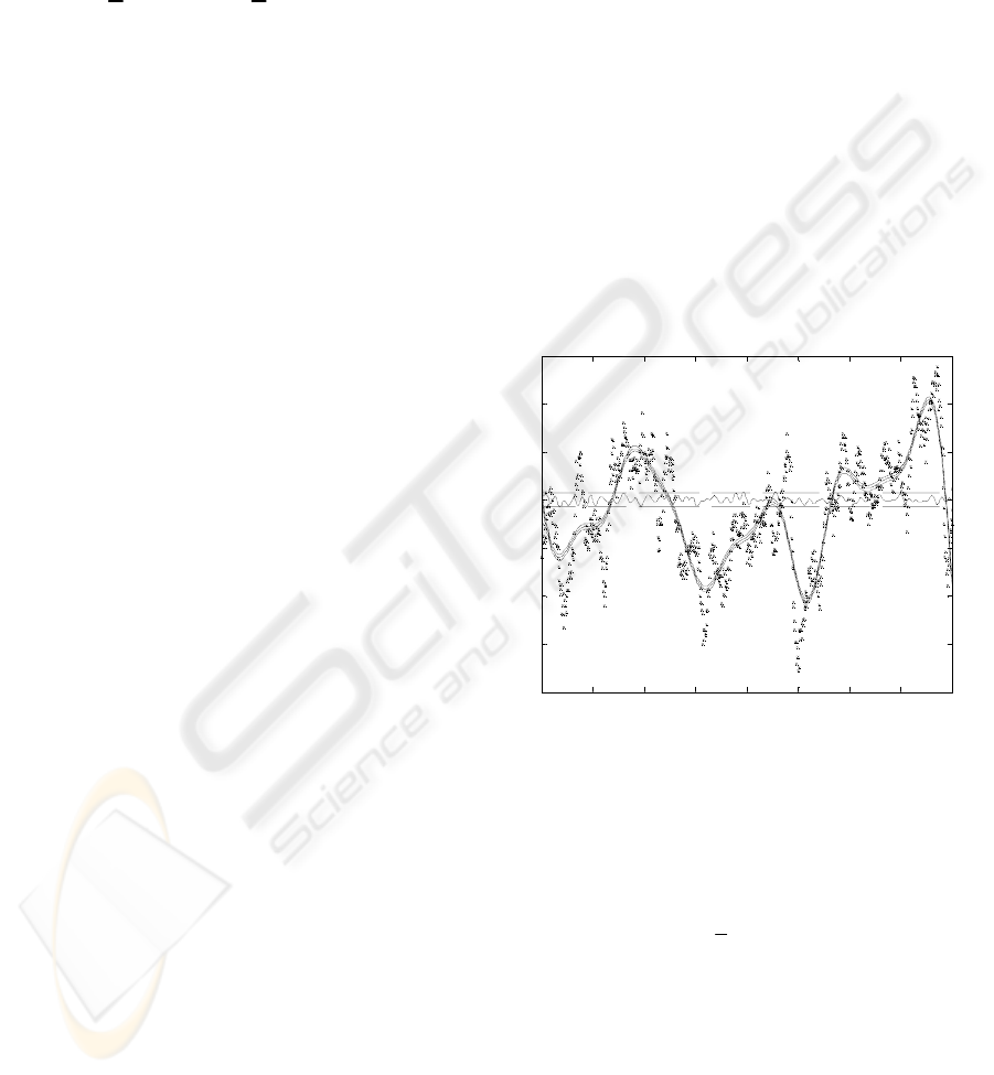
in Figure 3. The data has a long length-scale
component due to variations in the aerodynamic
torque, caused by changes in the wind speed and the
pitch angle of the rotor blades, and a short length-
scale component due to the structural and electro-
mechanical dynamics of the machine. From Figure
3, these two components can be clearly seen as can
the poor quality of the data.
200 220 240 260 280 300 320 340 360 380 400
24.5
25
25.5
26
26.5
27
27.5
Data
Seconds
Figure 3: Rotor speed measurements from 200s to 400s
265 266 267 268 269 270 271 272 273 274 275
24.5
25
25.5
26
26.5
27
27.5
Long-length scale prediction and confidence intervals
Seconds
Data
Prediction
Std Dev
Figure 4: Rotor speed prediction, confidence intervals and
data from 265s to 275s
200 220 240 260 280 300 320 340 360 380 400
24.5
25
25.5
26
26.5
27
27.5
Long-length scale prediction and confidence intervals
Seconds
Figure 5: Rotor speed prediction with confidence intervals.
WIND TURBINE ROTOR ACCELERATION: IDENTIFICATION USING GAUSSIAN REGRESSION
89
It is required to estimate the long-length-scale
component in the rotor speed. Since the structural
and electro-mechanical dynamics only induce small
oscillations in the measured values, a prediction of
the rotor speed using (8) is appropriate with f
z
and g
z
the long and short-length components respectively.
The covariance function for f
z
is chosen to have the
form (9) with hyperparameters a
f
and d
f
as is the
covariance function for g
z
with hyperparameters a
g
and d
g
. The measurement noise is assumed to be
Gaussian white noise with variance b. Hence, the
prior covariance for the measurements, y
i
, at time, t
i
,
are
ij
bda
da
δ
+−−+
−−=
])tt(exp[
])tt(exp[]y,y[E
2
jig
2
1
g
2
jif
2
1
fji
(13)
Given the data, the hyperparameters are adapted to
maximize the likelihood. Since there are 24,000 data
values, it is necessary to use the vector-storage
Toeplitz algorithms of Section 4.2.
200 220 240 260 280 300 320 340 360 380 400
-1.5
-1
-0.5
0
0.5
1
1.5
Derivative prediction with confidence intervals
Seconds
Figure 6: Derivative prediction with confidence intervals
265 266 267 268 269 270 271 272 273 274 275
-1.5
-1
-0.5
0
0.5
1
1.5
Derivative prediction with confidence intervals
Seconds
Figure 7: Derivative prediction with confidence intervals
A section, from 200s to 400s, of the prediction for
the rotor speed, i.e. the long length-scale component,
together with the confidence intervals is shown in
Figure 5 and a typical short section, from 265s to
275s, in Figure 4. From the latter, it can be seen that
the rotor speed has been successfully extracted.
However, it is not the rotor speed per se that is of
interest but its derivative. A section, from 200s to
400s, of the prediction for the derivative of the rotor
speed together with the confidence intervals is
shown in Figure 6 and a short section, from 265s to
275s, in Figure 7.
6 CONCLUSIONS
From poor quality wind turbine rotor speed
measurements, the rotor speed and acceleration are
estimated within narrow confidence intervals using
Gaussian process regression. To do so, two issues
are addressed. Firstly, the rotor speed is extracted
from a combined rotor speed and generator speed
measurement. A novel adaptation of Gaussian
process regression based on two independent
processes rather than a single process is presented.
Secondly, efficient algorithms for the manipulation
of large matrices (24,000x24,000) are required. The
Toeplitz nature of the matrices is exploited to derive
novel fast algorithms for the Gaussian process
methodology that are memory efficient.
ACKNOWLEDGEMENTS
This work was supported by Science Foundation
Ireland grant, 00/PI.1/C067, and by the EPSRC
grant, GR/M76379/01
.
REFERENCES
Gibbs, M. N., 1997. Bayesian Gaussian processes for
regression and classification, Ph.D. thesis, Cambridge
University.
Gibbs, M. N., and Mackay, D. J. C., 2000. Variational
Gaussian process classifiers, IEEE Transactions on
Neural Networks, Vol. 11, pp. 1458-1464.
Golub, G. H., and Van Loan, C. F. , 1996. Matrix
Computations. Baltimore: Johns Hopkins University
Press.
Leith, D. J., Leithead, W. E., Solak, E., and Murray-
Smith, R., 2002. Divide and conquer identification
using Gaussian process priors, Proceedings of the 41st
ICINCO 2005 - SIGNAL PROCESSING, SYSTEMS MODELING AND CONTROL
90

IEEE Conference on Decision and Control, Vol. l 1,
pp. 624-629.
Leithead, W. E., Solak, E., and Leith, D., 2003a. Direct
identification of nonlinear structure using Gaussian
process prior models, Proceedings of European
Control Conference, Cambridge.
Leithead, W. E., Hardan, F., and Leith, D. J., 2003b,
Identification of aerodynamics and drive-train
dynamics for a variable speed wind turbine,
Proceedings of European Wind Energy Conference,
Madrid.
Leithead, W. E., Kian Seng Neo, Leith, D. J., 2005.
Gaussian regression based on methods with two
stochastic processes, to be presented, IFAC, Prague,
2005.
Mackay, D. J. C., 1998. Introduction to Gaussian
processes. In Neural Networks and Machine Learning,
F: Computer and Systems Sciences (Bishop, C. M.,
Ed.), Vol. 168, pp. 133-165, Springer: Berlin,
Heidelberg.
O’Hagan, A., 1978. On curve fitting and optimal design
for regression, J. Royal Stat Soc. B, 40, pp. 1-42.
Rasmussen, C. E., 1996. Evaluation of Gaussian processes
and other methods for non-linear regression, Ph.D.
thesis, University of Toronto.
Sambu, S., Wallat, M., Graepel, T., and Obermayer, K.,
2000. Gaussian process regression: active data
selection and test point rejection, Proceedings of the
IEEE International Joint Conference on Neural
Networks, Vol. 3, pp. 241-246.
Shi, J. Q., Murray-Smith, R., and Titterington, D. M.,
2003. Bayesian regression and classification using
mixtures of multiple Gaussian processes, International
Journal of Adaptive Control and Signal Processing,
Vol. l 17, pp. 149-161.
Solak, E., Murray-Smith, R.,. Leithead, W. E., Leith, D.,
and Rasmussen, C. E., 2003. Derivative observations
in Gaussian process models of dynamic systems,
Advances in Neural Information Processing Systems,
Vol. 15, pp. 1033-1040, MIT Press.
Williams, C. K. I., 1999. Prediction with Gaussian
processes: from linear regression to linear prediction
and beyond, Learning in Graphical Models (Jordan,
M. I., Ed.), pp. 599-621.
Williams, C. K. I., and Barber, D., 1998. Bayesian
classification with Gaussian processes, IEEE
Transactions on Pattern Analysis and Machine
Intelligence, Vol. l 20, pp. 1342-1351.
Yoshioka, T., Ishii, S., 2001. Fast Gaussian process
regression using representative data, Proceedings of
International Joint Conference on Neural Networks,
Vol. l 1, pp. 132-137.
WIND TURBINE ROTOR ACCELERATION: IDENTIFICATION USING GAUSSIAN REGRESSION
91
