
ON-LINE SUPERVISED ADJUSTMENT OF THE CORRECTING
GAINS OF FRACTIONAL ORDER HOLDS
A. Bilbao-Guillerna, M. De la Sen and S. Alonso-Quesada
Instituto de Investigación y Desarrollo de Procesos, Facultad de Ciencia y Tecnología,
Universidad del País Vasco, Aptdo. 644 de Bilbao, 48080-Bilbao (Spain)
Keywords: FROH, multimodel, switching techniques.
Abstract: A discrete control using different possible discretization models of a continuous plant is presented. The
different models of the scheme are obtained from a set of different discretizations of a continuous transfer
function under a fractional-order-hold of correcting gain [1,1]
β
∈
− (β-FROH). The objective is to design a
supervisory scheme which is able to find the most appropriate value for the gain β in an intelligent design
framework. A tracking performance index evaluates each possible discretization and the scheme chooses the
one with the lowest value. Two different methods of adjusting this value are presented and discussed. The
first one selects it among a fixed set of possible values, while in the second one the value of
β
can be
updated by adding or subtracting a small quantity. Simulations are presented to show the usefulness of the
scheme.
1 INTRODUCTION
This paper deals with the problem of controlling a
known continuous plant using an appropriate
discrete controller selected from a group of possible
ones. Each possible controller is associated to a
different discretization of the plant (Alonso-Quesada
and De la Sen, 2004; Broeser, 1995; Ibeas et al.
2002; Middleton et al. 1988; Narendra and
Balakrishnan, 1995 and 1998). A fractional order
hold is used in order to generate the continuous input
from the discrete signal. The choice of the
β
gain
of the FROH device should be taken into account,
since the discretization zeros depend on its election
(Åström and Wittenmark, 1984; Bárcena et al.,
2000; Ishitobi, 1996). In order to find the most
appropriate discretization of the continuous plant,
two different methods are proposed. In the first one,
a set of fixed values of
β
are used to generate a
group of discretization models. Obviously, only one
value of
β
can be used at each time, but since the
plant is supposed to be known we can simulate the
behavior of all the possible discretization. A tracking
index evaluates the performance of all of them and
the system uses the one with the lowest value to
implement the FROH device and the control law. In
the second method, we only allow the system to
update the value of
β
to a close one. The behavior
of the current discretization is compared with the
behavior of other two possible discretizations. One
model using a gain
β
being slightly larger and the
other one using a
β
being a bit smaller. The second
method has a slower convergence to an optimum
value of
β
, but it avoids the transient in the output
which may occurred when
β
is changed a large
value. Some computer simulations about two
practical cases will be given in order to highlight the
usefulness of the proposed multi-model scheme. In
the first case, a DC motor is simulated. In the second
one, we deal with a LCR parallel circuit (Tank
circuit).
2 PROBLEM DESCRIPTION
In this paper, we are dealing with the problem of
controlling a continuous plant by using a set of
discrete controllers. Each of those controllers is
associated to a different discretization of the
continuous plant under a fractional order hold
(FROH) with a correcting gain β. The plant
continuous input signal obtained from a β-FROH
follows this equation,
266
Bilbao-Guillerna A., De la Sen M. and Alonso-Quesada S. (2005).
ON-LINE SUPERVISED ADJUSTMENT OF THE CORRECTING GAINS OF FRACTIONAL ORDER HOLDS.
In Proceedings of the Second International Conference on Informatics in Control, Automation and Robotics - Robotics and Automation, pages 266-271
DOI: 10.5220/0001178302660271
Copyright
c
SciTePress
()
1
()
kk
ks
s
uu
ut u t kT
T
β
−
⎡⎤
−
=+ −
⎢⎥
⎣⎦
(1)
for
()
1
s
s
kT t k T≤< + , where
s
T is the sampling
time,
[1,1]
β
∈− and ()
ks
uukT= is the input signal
to the hold at
s
tkT= for each integer 0k ≥ . For
0
β
= and 1
β
= the zero-order-hold (ZOH) and the
first-order-hold (FOH) are obtained respectively.
The discrete transfer function of a continuous one,
()
()
()
Ns
Gs
Ds
=
, results to be as follows,
() ()
() () () ()
() ()
Ns Bz
Hz Z h s Gs Z h s
Ds Az
ββ
⎡⎤
⎡⎤
=⋅= ==
⎢⎥
⎣⎦
⎣⎦
1
10
1
10
...
...
mm
mm
nn
n
bz b z b
zaz a
−
−
−
−
+++
+++
(2)
where,
(1 ) 1
() 1
s
s
s
s
TsT
sT
s
ee
hs e
Ts s
β
β
β
−−
−
⎛⎞
−−
=− +
⎜⎟
⎝⎠
is
the transfer function of a β-FROH, Z the Z-transform
and the polynomial degrees,
deg( ) 0
deg( )
deg( ) 1 0
Dif
nA
Dif
β
β
=
⎧
==
⎨
+≠
⎩
and
deg( )mB= . Moreover, 1nm=+ if
deg( ) deg( )ND< or nm
=
if deg( ) deg( )ND= .
Since the use of a ZOH is more common in practice
than the use of a FROH,
()
H
z may be calculated
just using ZOH devices in the following way,
[]
00
(1) ()
() () () ()
s
zzGs
Hz Zh s Gs Z h s
zTzs
ββ
−−
⎡⎤
=⋅+ ⋅
⎢⎥
⎣⎦
(3)
where,
0
1
()
s
T
e
hs
s
−
−
=
is the transfer function of a
ZOH device. The following standard assumptions
are made:
1-It is assumed that both polynomials
()Ns and
()Ds are known.
2-The reference model,
/
mmm
H
BA= , is
exponentially stable, i.e. all the roots of
m
A
satisfy
1z
δ
≤− for some
(
]
0,1
δ
∈ .
3-There exists a known convex and compact subset
2n
D ⊆ℜ of the parameter space where the real
parameter vectors belong to so that for all plant
parameterization in D the polynomials A and B are
coprime.
2.1 Basic adaptive controller
The transfer function of the reference model is,
'
00
00
() () ()
()
() ()
mm
m
mm
BzBzAz BA
Hz
A
zA z AA
−
== (4)
where
'
()
m
Bz
contains the free-design reference
model zeros, ()Bz
−
is formed by the
unstable(assumed known) plant zeros and
0
()
A
z is a
polynomial including the eventual closed-loop stable
pole-zero cancellations which are introduced when
necessary to guarantee that the relative degree of the
reference model is non less than that of the closed-
loop system so that the synthesized controller is
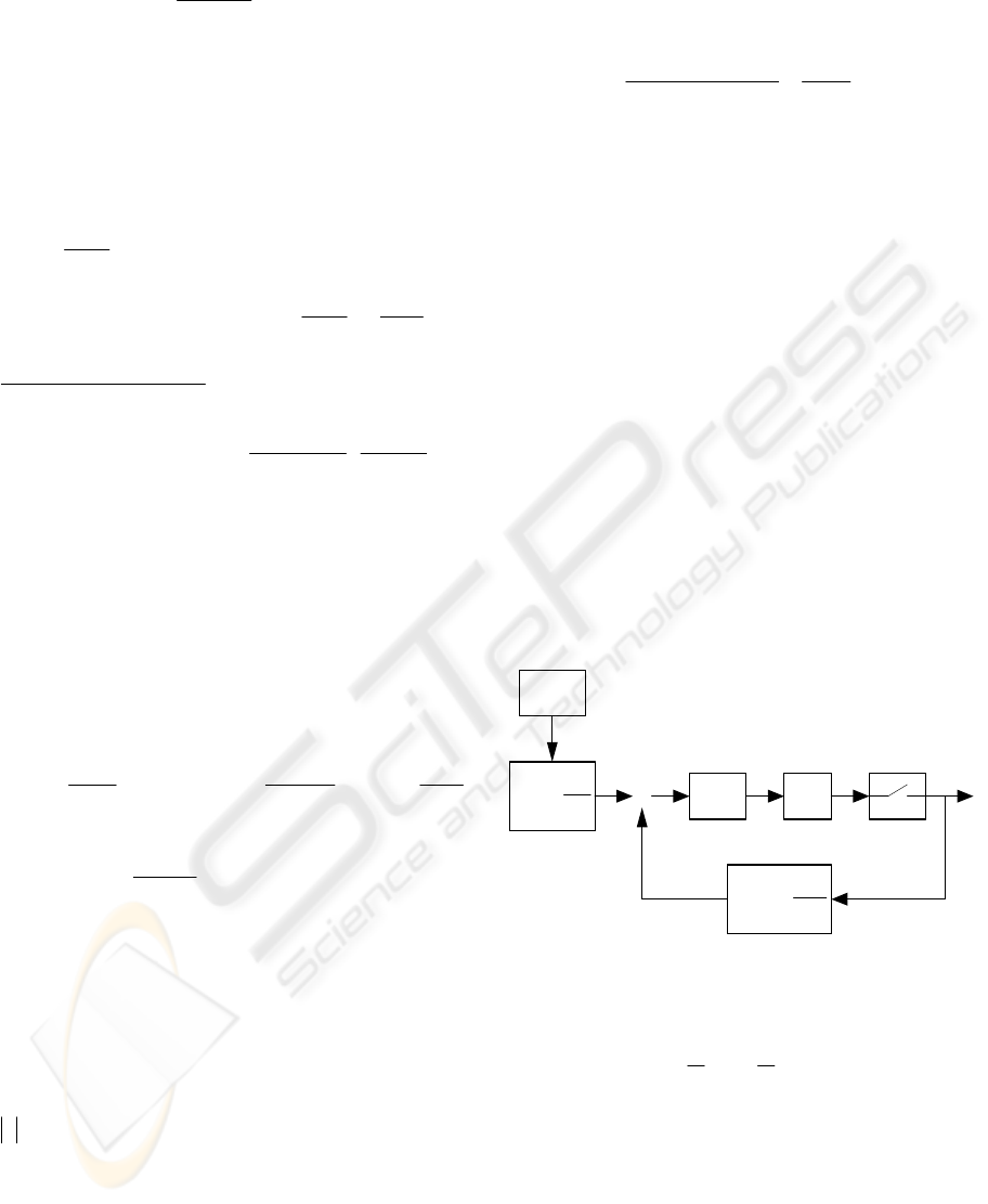
causal. A basic control scheme is displayed in figure
2. Then, we will consider the polynomials
k
R ,
k
S
and
T
(T depends only on the reference model zeros
polynomial which is of constant coefficients) where
'
0m
TBA= and
k
R (monic),
k
S are the unique
solutions with degrees fulfilling
(
)
deg 2
k
Rni
=
− ,
(
)
deg 1
k
Si=−,
()
0
deg 2
m
A
An=
of the polynomial diophantine equation
01, 0kk kk k m k k k m
A
R BS BAA AR BS AA
+−
+= ⇔ += (5)
with
1,kkk
RBR
=
at every sampling instant. Figure 1
shows the control scheme.
Reference
Input
⊗
FROH G(s)
()
()
()
ff
Tz
Hz
R
z
=
()
()
()
fb
Sz
Hz
R
z
=
,ck
u
k
y
()yt
k
u
()ut
+
−
s
T
Figure 1: Basic control scheme
From (4)-(5), perfect matching is achieved through
the control signal:
,kckk
TS
uu y
RR
=−
(6)
2.2 Multimodel scheme A
In order to find the most appropriate value of the
gain
β
, we consider a set of possible design values
of it and the corresponding discrete transfer function
is obtained,
ON-LINE SUPERVISED ADJUSTMENT OF THE CORRECTING GAINS OF FRACTIONAL ORDER HOLDS
267

()
() ()· ()
H
zZhsGs
β
⎡⎤
=
⎣⎦
A
A
for 1
m
n≤≤A (7)
where
m
n is the number of possible values of
β
and
()
β
A
is used to indicate its value for the
th
A model.
Once all the possible discrete transfer function are
obtained for the whole set of intended values, we can
simulate the performance of all of them when the
previous control law is applied and compared their
responses with the desired reference output.
()
m
Gs
()Gs
(1)
()FROH
β
()Gs
()Gs
(2)
()FROH
β
()
()
m
n
FROH
β
#
⊗
⊗
⊗
()
c
ut
1,k
u
2,k
u
,
m
nk
u
1
()ut
2
()ut
()
m
n
ut
()
m
yt
1
()yt
2
()yt
()
m
n
yt
1
()et
2
()et
()
m
n
et
+
+
+
−
−
−
Figure 2: Multimodel scheme
Each plant input is generated by using the control
law (6), where the reference transfer function (4),
which should be matched, is the corresponding
FROH discretization of
()
m
Gs. In other words, we
have as many reference transfer functions as the
number of possible values of
β
we are considering.
2.3 Switching rule and identification
performance index
The objective of the supervisor is to evaluate the
tracking performance of the possible controllers
operating on the plant for the given reference model
with the aim of choosing the current controller from
the set of parallel controllers. The proposed
performance index is:
()
()
(1)
() ()
s
s
k
jT
kj
km
jT
jkM
J
yyd
λ
τττ
−
−
=−
=−
∑
∫
A
A
(8)
for
1
m
n≤<A , where, (0,1]
λ
∈ and 0M > are
design real parameters.
λ
is a forgetting factor
which allows us to give more importance to the last
time interval.
2.4 Multimodel scheme B
In this case, instead of letting the system to choose
among any of the possible values of
β
, we only
allow the system to change to a close value. The
system starts with an arbitrary value and the tracking
performance is compared with the tracking
performance of two possible close values of
β
. One
being a bit larger and the other one a bit lower. With
this method, when we compare their responses, the
system can only choose among three possible cases.
In other words, n
m
is always three. However, these
three possible values are not going to be constant
and they are updated. If the system chooses one of
the two close values of
β
, then it becomes the
active one and the other two are chosen by adding
and subtracting a quantity to it. If the system chooses
to maintain the same value of
β
, then the other two
possible values are updated as well by considering
other two closer values of
β
. In order to explain
this method, the following algorithm describes how
it works,
a) At
th
k
sample the active value of
β
is
k
β
. Other
two values,
sup
kk
βββ
=
+∆ and
inf
kk
βββ
=−∆ are
used for simulation. Suppose that the last
β
switching took place at
th
k sample.
b) If
(1)kTkTMT+−≥ , then the tracking
performance of the three possible discretizations are
compared and the one with the lowest value of (8) is
used in the FROH device.
c) If the system chooses to maintain the same value
of
β
, first
β
∆
is decreased and then
sup
β
and
inf
β
are updated.
- if
1kk
ββ
+
=
then / mf
ββ
∆
=∆ (with 1mf > ) and
sup inf
11
,
kk kk
ββββββ
++
=
+∆ = −∆
d) If the system chooses another value,
β
∆
maintains its value and
sup
β
and
inf
β
are calculated
by adding and subtracting this value
- if
sup
1kk
ββ
+
= then
sup
1
2
kk
ββ β
+
=
+∆,
inf
1kk
ββ
+
=
- if
inf
1kk
ββ
+
= then
sup
1kk
ββ
+
=
,
inf
1
2
kk
ββ β
+
=−∆
Note that there are two supervisory hierarchized
levels of action of this intelligent system, namely:
1)
The basic control: It consists of generating
via u
k
from (5) for each of the discrete
models integrated in the multi-model
scheme.
2)
The choice of
β
: The model and gain
β
of the FROH is on-line selected by a
switching rule via minimization of the
supervisory performance index (8).
ICINCO 2005 - ROBOTICS AND AUTOMATION
268
3 SIMULATION RESULTS
In this section two different cases are presented in
order to show the usefulness of the proposed
scheme. The first one simulates a DC motor, while
the second one deals with a resonant circuit. In both
cases, the two different multi model methods are
used.
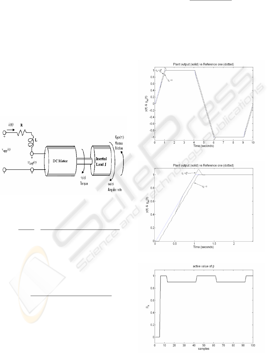
3.1 DC motor
A simple model of a DC motor driving an inertial
loads shows the angular rate of the load,
()wt , as the
output and applied voltage,
()
app
vt, as the input. The
objective is to control the angular rate by varying the
applied voltage (Krishnan, 2001). Fig 3 shows a
standard model of the DC motor.
Figure 3: DC motor model
The transfer function of a DC motor can be
described as:
2
()
()
() ( )
m
app
ffbm
k
ws
Gs
vs LJs LK JRsRKkk
==
++++
The simulation is done by using the following
parameters,
0.5R =Ω, 1.5LmH= , 0.05 /
m
kNmA= ,
2
0.00025 / /
J
Nm rad s= , 0.0001 / /
f
kNmrds= ,
0.025 / /
b
kVrads= , which give the continuous
transfer function,
72
0.05
()
3.75·10 0.0001252 0.0013
Gs
ss
−
=
++
The first simulation uses the first multimodel case.
The set of possible gains
β
are:
()
1( 1)/10
i
i
β
=− − for 121i≤≤
The sampling time is chosen 0.1s and the residence
time is 5 samples. The reference output is obtained
from the following continuous transfer function,
2
500000
()
200 12500
m
Gs
ss
=
++
Figures 4 shows the plant output when the
β
value
is maintained fixed and when it is updated. The
dotted line indicates the desired reference output.
Figure 5 shows the active value of
β
during the
whole simulation. It is obvious that the tracking
performance is improved by selecting an appropriate
value of the gain
β
.
Figure 4 a: Plant output with method A
Figure 4 b: Plant output with method A (zoom over first
seconds)
Figure 5: active value of
β
with method A
ON-LINE SUPERVISED ADJUSTMENT OF THE CORRECTING GAINS OF FRACTIONAL ORDER HOLDS
269
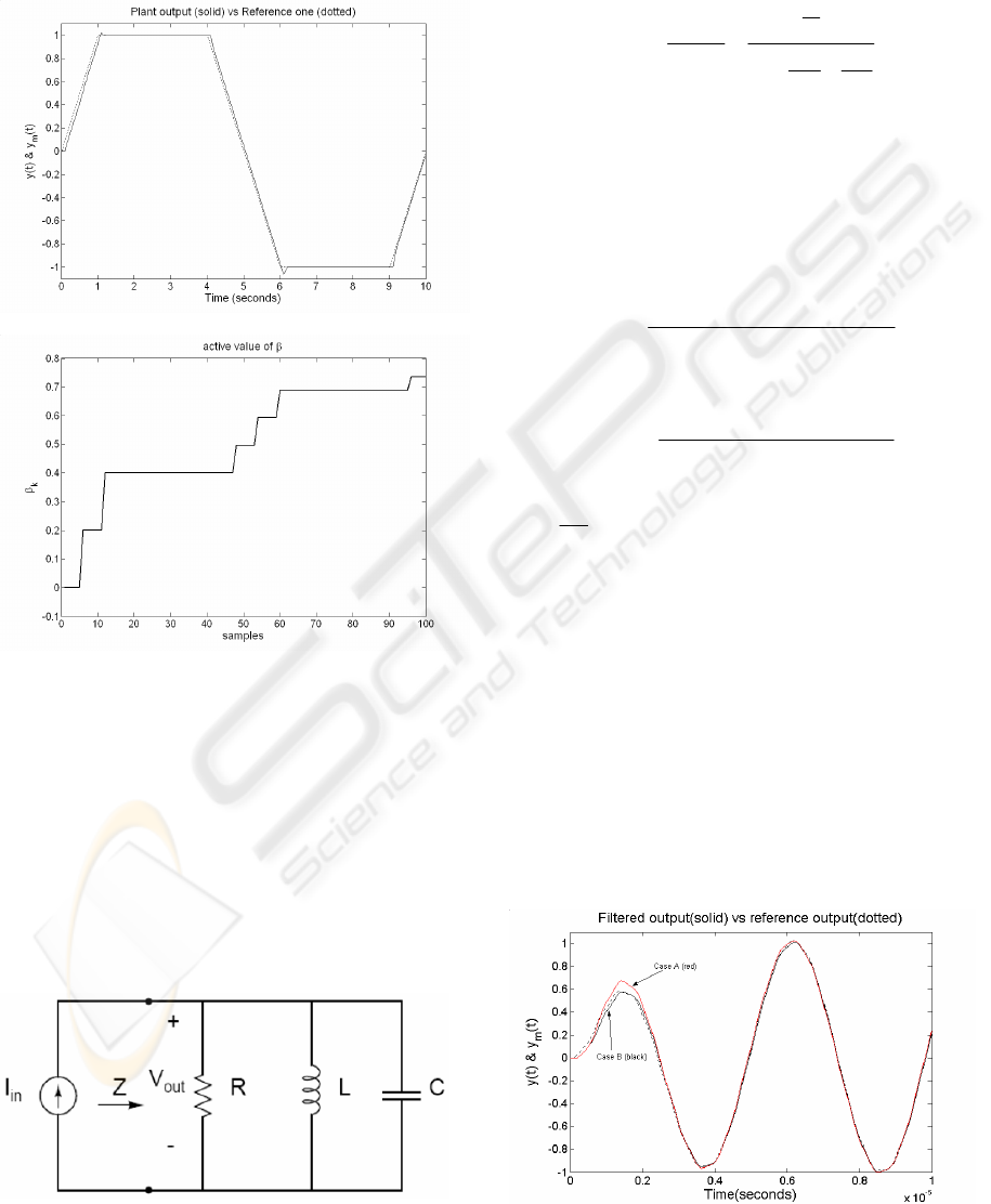
The simulation is repeated with the second
multimodel method. Figure 6 shows the plant output
and figure 7 the on-line active value of
β
selecting
via switchings using (8). The initial value for
β
∆
is
0.2 and m
f
is 1.2.
Figure 6: Plant output with method B
Figure 7: Active value of
β
with method B
In this case, it takes more time to achieve a good
value of
β
as we do not let it to take the best one in
the first switching. One could think that this is a bad
option. However, next simulation will show that
sometimes this method have a better performance.
3.2 Resonant Circuit (Tank Circuit)
A resonant circuit is simply an LCR circuit with a
zero-pole cancellation at
0s = at the resonance
frequency (Floyd, 2003).
Figure 8: Parallel RLC circuit
Usually the effect of the resistance is small
compared to the size of the inductance and the
capacitance. This leads to highly resonant behavior.
In this work, we will consider a parallel RLC circuit
with a transfer function,
2
()
()
1
()
out
in
s
Vs
C
Gs
s
Is
s
RC LC
==
++
The resonant frequency
m
w of a resonant circuit is
the frequency corresponding to the peak value of the
transfer function and it occurs when
1/
m
wLC= .
Simulations are performed for a circuit with
parameters
100R
=
Ω , 2LmH
=
and 300CpF= .
Replacing these values, the transfer function results
to be:
7
2712
3.333·10
()
3.3333·10 1.667·10
s
Gs
ss
=
++
The reference output is obtained from the following
continuous transfer function:
6
26 12
1.667·10
()
1.667·10 1.667·10
m
s
Gs
ss
=
++
The resonant frequency is located in
205
2
m
m
w
fkHz
π
== . Both multi-model schemes
with the same parameters as in previous section are
simulated. The reference input is generated as the
sum of four of four sinusoidal signals of different
frequencies {0.1w
m
, w
m
, 10w
m
, 100w
m
}. It is suited
for the circuit to select the one at the resonant
frequency. Figure 9 shows the plant output in both
cases together with the reference output. In this case,
although both outputs tend to the desired one, the
second multi-model has a better transient behavior in
the first time interval. This occurs, because when we
change the value of
β
in a big quantity, the plant
behavior suffers a little transient as it can be shown.
However, with small changes this transient is found
to be smaller.
Figure 9: Plant outputs using method 1 and 2
ICINCO 2005 - ROBOTICS AND AUTOMATION
270

Finally, figures 10 and 11 show the active value of
β
in both simulations.
Figure 10: Active value of
β
with method 1
Figure 11: Active value of
β
with method 2
4 CONCLUSIONS
In this paper, a multi-model based discrete control
scheme for a continuous plant has been presented.
The different discrete models are obtained by
discretizing the continuous plant under a FROH
device. The scheme is designed to find the value of
the gain
β
which leads to the best tracking
performance. Two different methods have been
presented for this purpose. The first one selects the
current value of the gain among a fixed set of
possible values. The second one updates
β
only to a
close value, avoiding bad transients which may
occur when the changing is big. Finally, the
proposed schemes have been used in two practical
cases. Simulations showed that an appropriate
choice of the value of
β
leads to a good tracking
performance, even if a continuous plant is under
control by a discrete controller. Moreover, the
advantages and disadvantages of both methods have
been figured out through the simulation results.
ACKNOWLEDGEMENTS
The authors are very grateful to MEC and UPV by
partial supports through Research Grants DPI 2003-
00164 and Scholarship of A.Bilbao BES-2004-4261,
and 9/UPV 00I06.I06-15263/2003.
REFERENCES
Alonso-Quesada, S. and De la Sen, M., 2004. ‘Robust
Adaptive Control with Multiple Estimation Models for
Stabilization of a Class of Non-inversely Stable Time-
varying plants’, Asian Journal of Control, Vol. 6, Nº
1, pp. 59-73.
Åström, K.J. and Wittenmark, B., 1984. ‘Zeros of
Sampled Systems’, Automatica, 20, 31-38.
Bárcena, R., De la Sen, M. and Sagastabeitia, I., 2000
‘Improving the Stability of the Zeros of Sampled
Systems with Fractional Order Hold’, IEE Proc.
Control Theory and Applications, 147, Vol. 4, pp.456-
464.
Broeser, P.M.T., 1995. ‘A Comparison of Transfer
Functions Estimators’, IEEE Transactions on
Instrumentation and Measurement, Vol. 44, Nº 3,
pp.657-661.
Floyd, T., 2003. ’Electronic Circuits Fundamentals’,
Prentice Hall.
Ibeas, A., De la Sen, M. and Alonso-Quesada, S., 2002. ‘A
Multiestimation Scheme for Discrete Adaptive Control
which Guarantees Closed-loop Stability’, Proc. of the
6
th
WSEAS Multiconference on Systems, pp.6301-
6308.
Ishitobi, M., 1996. ‘Stability of Zeros of Sampled Systems
with Fractional Order Hold’, IEE Proc., Control
Theory and Applications, 143, pp. 296-300.
Krishnan, R., 2001. ‘Electronic Motor Drives: Modelling,
Analysis and Control. Book 1’, Prentice Hall.
Middleton, R.H., Goodwin, G.C. Hill, D.J and Mayne,
D.Q., 1988. ‘Design Issues in Adaptive Control’, IEEE
Transactions on Automatic Control, Vol. 33, Nº 1,
pp.50-58.
Narendra, K. S. and Balakrishnan, J., 1994. ‘Improving
Transient Response of Adaptive Control Systems
using Multiple Models and Switching’, IEEE
Transactions on Automatic Control, Vol. 39, No. 9,
pp. 1861-1866.
Narendra, K. S. and Balakrishnan, J., 1997 ‘Adaptive
Control Using Multiple Models”, IEEE Transactions
on Automatic Control, Vol. 42, No. 2, pp. 171-187.
ON-LINE SUPERVISED ADJUSTMENT OF THE CORRECTING GAINS OF FRACTIONAL ORDER HOLDS
271

ICINCO 2005 - ROBOTICS AND AUTOMATION
272
